Building Meaning From Data
Modern Tools for Working with Data
The term Data Science is ubiquitous, and definitions vary. This is similar for terms such as informatics, bioinformatics, computational biology, among others. The terms are largely generic, but the underlying concepts are largely the same and do not change fully. It’s important to give a few areas, we will focus on:
- BASH/Command-line
- Python. A general-purpose scripting/programming language that emphasizes code readability.
- R. A scripting language with its routes in statistics
- Databases (SQL). A standard language for accessing and manipulating databases.
In any job function that are many tools. We focus largely on two: R and Python. There is a lot of debate between those that are experts in one or the other. Like with anything, it all depends on context and purpose. If you had to analyze a dataset in 24 hours to get the first idea of significant findings and a standard vignette existed in R, you would probably be better served using R. Likewise, if python programs and modules existed in Python for an analysis, you might pick Python. In the end, this all starts with goals and follows a series of standard questions:
- What is your primary goal?
- What is your timeline?
- Are there standard tools or best practices?
There are a few counter-intuitive approaches most experienced individuals use when taking on a new analysis:
- Start with standard and established best practices, workflows, and vignettes, then modify iteratively based on your own objectives.
- Take this a step further: Verify these best practices using unit-test data where possible, then modify code to incorporate your own objectives. Create as little novel code as possible.
- Iteratively develop analysis – live the Agile Manifesto.
Understanding the Types of Data
It’s important to start with the idea that we have different types of data. Data can be numbers, letters, dates, and so forth. Within a computer, these are all represented differently and in very defined ways.
Don’t Assume Two Times Two is Four
It’s a blustery cold night. You turn on the news station and listen to the weather. The weather person tells you: “It’s cold at 2C, but not to worry, temperatures will double by morning to 4C.”
Lets think about that. If the temperature doubles, well we can then say `2C * 2 = 4C`
Lets break that down. We have a measurement, `2C` and we have an operator: `*`. The question in front of you: Is multiplication of centigrades a valid operation?
If we take the example above and convert to Farhenheight, we see something isn’t right. In Farhenheight, 2C is 35.6 and 4C is 39.2. Clearly 2*35.6F is not the same as 39.2.
What’s the difference between the number 2, the character 2, two, 2.0, 200%? Quite a bit, and the impact is significant to scientific data and data analysis. Recently, in fact, there was an article:
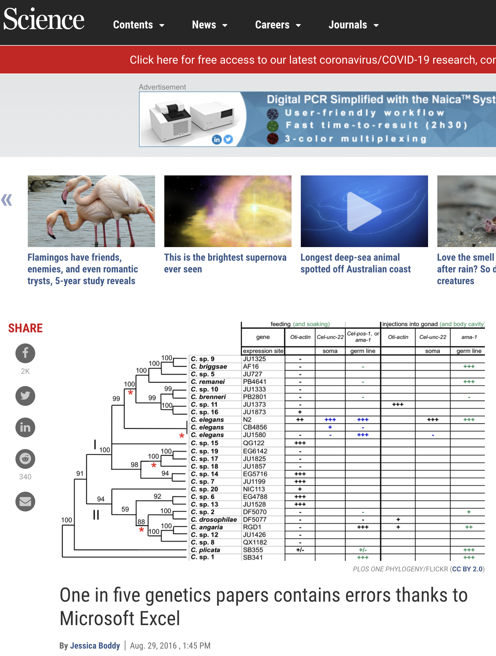
How can this arise? Open Excel and type the gene SEPT6and save it as a csv. For example, if we take a file and put:
Gene, Value
KRAS, 2.323
SEPT6, 2321
TP53, 2.1.2
Then we open it excel and see that the data has changed. This can have far-reaching effects, and is something to be careful:
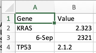
We then save it, and look at the raw data we see that the underlying data has changed.
Gene, Value
KRAS,2.323
6-Sep,2321
TP53, 2.1.2
What’s happening is that Excel is interpreting and determining the type of the data, and decides that SEPT6 should be a date. In Excel, date is a type of data. Accordingly, it then stores it in a way whereby fundamentally it’s changed. Excel is what’s called a weak type language, and guesses what type of data is underlying. Other languages are strong typed. What does this mean, and what are some fundamental types? We review a few, but its important to understand each language has types and these are some of the most primordial parts of data science we need to understand.
Primitive or Simple Data types
We first describe the basis for primitive datatypes.
Bits & boolean types of data
A bit is the basic unit of data that is either 0 or 1. Everything builds from there. A common representation is true/false (boolean).
Boolean is the first type of data to remember, and it can be encoded as a 0 or 1.
We can describe more complex data by using bits together. Two bits give us access to four slots:
| 00 | Slot 1 |
| 01 | Slot 2 |
| 11 | Slot 3 |
| 10 | Slot 4 |
We can extend this further to 8 bits and beyond
8 Bits to a Byte & a character or char type of data.
Modern computing really began when we started using 8 bits to represent a byte of data. 2^8 gives 256 categories. This is convenient because it can store what can be typed on a keyboard. The ASCII standard is the encoding of characters using 7 bits to these keys (below), reserving the last bit, and another 128 characters for foreign characters using the last 8th bit. Below we can see that A is 011 0001.
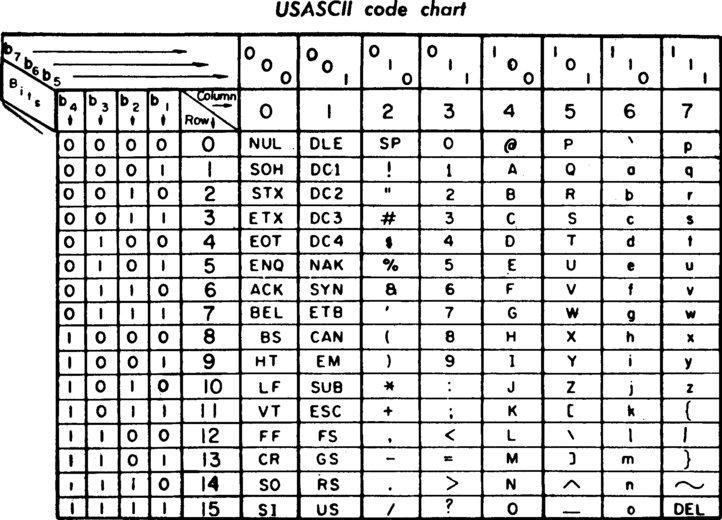
The second type of data to know is character or sometimes abbreviated as char. It is a single letter. Character data types are typically strings of ASCII characters
Stringing characters together & string types of data
If we take several characters and bundle (or string) them together we have the next important type of data: Stings. A string data type is a series of characters stored together. We store these together in variables and we’ll discuss this more later. An example of string is:
data
which underneath the hood is composed of for characters in order: d,a,t,a.
Text & Beyond ASCII
In ASCII, every letter, digits, and symbols that mattered to the English Language… they are represented as a number 0-127 (a-z, A-Z, 0–9, +, -, /, “, ! etc.) . For 128 to 255 its been the wild-west as those characters were used for all sorts of things.
Unicode
The Unicode was the attempt to create a single character set that could represent every characters in every imaginable language systems. This required a shift in how to interpret characters. And in this new paradigm, each character was an idealized abstract entity. Also in this system, rather than use a number, each character was represented as a code-point. The code-point example of U+00639, where U stands for ‘Unicode’, and the numbers are hexadecimal.
UTF-8
UTF-8 encoding standard took from the Unicode attempts to create something that achieved bigger goals. In UTF-8, every code-point from 0–127 is stored in a single byte. Code points above 128 are stored using 2, 3, and in fact, up to 6 bytes. Remember that each byte consists of 8 bits, and the number of allowed information increases exponentially with the bits used for storage. Thus with 6 bytes (and not necessarily always 6), one could store as many as 2⁴⁸ characters. The benefits of UTF-8 meant that nothing changed from the ASCII so far as the basic English character-set was considered.
UTF-16
Like you might expect UTF-16 uses 16 bits to encode Unicode characters. Java folks love these. Bad news is a loss of backward compatibility.
Numbers
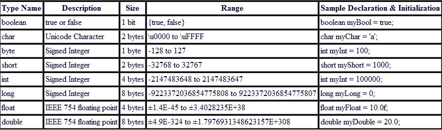
Using bits to represent whole numbers, integers as a type of data
Storing data has always been limiting – from floppy disks to IPads, nothing has changed – we need more storage. For example, consider the year 2020. We can store it as 4 char string:2020 . We can of course just abbreviate it as a year: ’20. For those old enough, they would immediately remember the year 2000 bug and the impact of such a decision. Essentially, for years prior to the year 2000, dates were stored using the last two digits, such as 99. As a result, the year 00 could either mean the year 1900 or 2000, and all downstream code had an inherent default prediction. This caused all sorts of challenges.
We can be smart about it though, and we can store it as a 2-bytes using 16 bits giving us access to 2^16=65,536 numbers. What if we want to store a larger number? We need to use a double integer that uses 4 bytes or 32 bits: 2^32=4,294,967,296. Building computers off of 32-bit computing was good throughout the 90’s when there were barely 5 billion people, but if we want the ability to go higher. Likewise, a genome is over 3 billion bytes, and if we store the location of a variant using 32 bits, we would lose precision and become ambiguous. We really need 64 bits: 2^64 gives us 18,446,744,073,709,551,616 numbers.
Using bits to represent numbers with decimals.
What about decimals? Well, we obviously would need more bits. A floating-point number is a limited-precision that is not whole and typically has a decimal. These numbers are stored internally as scientific notation. Still, floating-point numbers have limited precision, only a subset of real or rational numbers can be represented.
Float uses 8 bytes (or 64 bits) and gives us access to13.4^10-45 to 3.4^10+38. Need more, well, you need more bits.
Summary
Statistical Datatypes
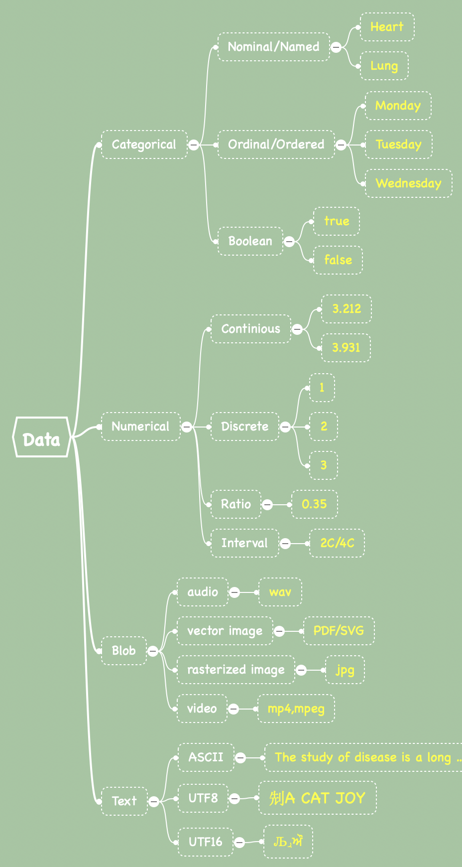
In many biomedical and data science applications, one is often interested in determining statistical meaning, it’s helpful to characterize the underlying data more and it can be sub-divided. By statistical meaning, we mean that we may wish to graph data, group data, or conduct statistical analysis on data. The first two major types of statistical data are categorical and numerical data (recognizing a few others as well, shown below).
Definitions vary by programming or scripting language, but generally, these are considered valid:
Categorical Data
Categorical data can take on one of a limited, and usually fixed, number of possible values, assigning each individual or other unit of observation to a particular group. Categorical data can then be typically divided into Ordinal/ordered data and un-ordered named or nominal data. Additionally, there is also boolean or binary data, that can be true or false. As many healthcare professionals now accept, gender is no longer binary.
Nominal Data
"Arizona","Nevada", "California"
Ordered Data
"Monday","Tuesday","Wednesday","Thursday"
Numerical Data
Numerical data is just that – data that is largely numbers. These take three primary forms: discrete, intervals , continuous, and ratio. Discrete data are usually considered whole numbers or integers, (such as 1,2,3,4), whereas continuous data can contain decimals. There is also a data-type called ratio that includes fractions and percentages, or types of data that really shouldn’t have some operations on them such as dividing. Another type are intervals which have a non-arbitrary zero, such as temperatures in the health-care setting would be temperature – going from 2C to 4C is not doubling in temperature. Other examples include enzyme activity, dose amount, reaction rate, flow rate, concentration, pulse, weight, and survival time.
|
Can be computed |
Nominal |
Ordinal |
Interval |
Ratio |
|
Equality |
Yes |
Yes |
Yes |
Yes |
|
Order |
No |
Yes |
Yes |
Yes |
|
Mode |
No |
No |
No |
Yes |
|
Frequency distribution |
Yes |
Yes |
|
Yes |
|
Median and percentiles |
No |
Yes |
Yes |
Yes |
|
Add or subtract |
No |
No |
Yes |
Yes |
|
Mean, standard deviation, standard error of the mean |
No |
No |
Yes |
Yes |
|
Geometric Mean |
No |
No |
No |
Yes |
|
Ratios, coefficient of variation |
No |
No |
No |
Yes |
Introducing variables & composite datatypes:
We are going to talk a lot about keeping data organized. We do this the same way we do in life – we give names to represents folders (both physical or otherwise), files, and just about everything else. Likewise, we put some data – whether an integer, character, or otherwise, we do want it back. We give them a name and box to be stored. They may change, and thus we use the term variable. Technically, there are also constants, but for our purposes, these are boxes where we store data and can retrieve them. We often type these variables so that the programs can optimally store them. An int variable may be able to store a single integer at a time. What about a set of data, such as a list of holidays? These can be stored as well in composite data types, such as arrays, dictionaries, or lists.
Collections of data can also be considered a single object and essentially a type of data. We review a few major types, but let’s start with considering a form of data as tables.
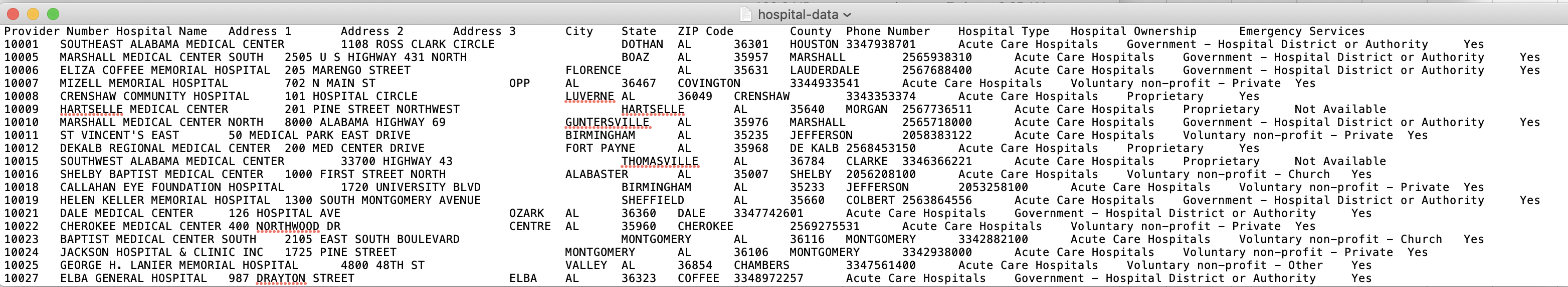
Composite Datatypes: Tables
Tables can be described through a spreadsheet Worksheet which most people are familiar with. Below, we have the table hospital-data with multiple column headers. This actually comes from a csv file (below) that is publicly available, and you can download it (link).
Arrays, Vectors, Lists, or Ordered Arrays.
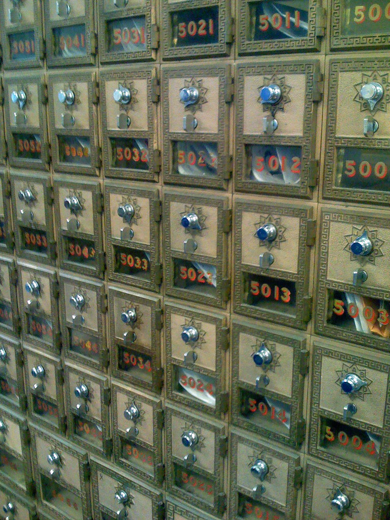
When we think of ways to store data, one analogy is by the mailbox. Basically, numbered places where we store data. If we think about a table from above, we could also consider an array to be a column.
Likewise, we can make an ordered list of data such as by A1 is ‘hello’ and A2 is ‘goodbye’. One might declare it (typically) by brackets. The key is that they are numbered sequentially. You can place things out of order, but in general, the expectation is that you push one thing onto a stack growing the size of the array by one.
A[1]=0.234234
A[2]=0.3234
A[3]=23.23
Arrays can, of course, be multi-dimensional, but generally, they are presumed to be all the same type of data, and thus you can write:
A[1,2]=0.234234
To emphasize, arrays are often indicated by brackets, and so when we see code or other types of data listed within brackets {}, then we should think of those as un-ordered arrays. For example:
workdays=["Monday","Tuesday","Wednesday","Thursday"]
We can then retrieve the first item in the list workdays[0] is Monday in some program languages and workday[1]. Indeed, some languages such as C start counting at 0 and some others such as R start at 1.
Associative arrays, Dictionaries, objects in javascript, named arrays, or hashes.
Number storage vehicles have limitations, and thus there is another type of storage that is much similar to an address, and those are termed Associative arrays. Instead of a number, we use a name.
GeneNames={"PTEN":"phosphatase and tensin homolog","KRAS":"K-Ras","TP53":"p53"}
I could have a variable called GeneNames. I could store GeneNames{'PTEN'}, and then store all sorts of information in a way that is logically retrievable. This comes in handy a lot. Again, historically, you do have the same type of data in unordered lists or hashes.
We can get much more complex and mix these quite a bit into data structures. In R, we use dataframes, which include Hashes of arrays, etc., and so forth. For example, let us load up some data!
These can be mixed where we have arrays of dictionaries and vice versa. We’ll get back to that point with JSON stores below.
Matrix
A matrix is a 2-dimensional grid of homogenous data without headers or row labels typically and is often used for matrix algebra.
Tensor
A tensor is a 3/n-dimensional cube of homogenous data. Tensors are typically used in deep neural networks in machine learning, which is where the deep learning framework TensorFlow gets its name.
 Graphs.
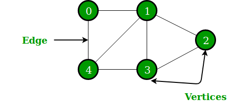
Data as a set of nodes and edges. Graphs are used to represent a network of data. They represent each item as a node and each relationship as an edge.
Tree
A tree organizes data as a set of nodes and branches. Trees are used to represent hierarchical data

Document Stores/Objects
JSON and Document Stores
JSON is a language-independent data format that allows for embedded data types of data, in a record. A collection of records is often called a document. At the heart of JSON is the Key:Value approach, where the value can strings, booleans, numbers, arrays, associative arrays, and null. Strings are encapsulated in quotes ("), boolean is unquoted true or false , arrays are surrounded by brackets, [and ], Associative arrays are surrounded by curly brackets, { and }.
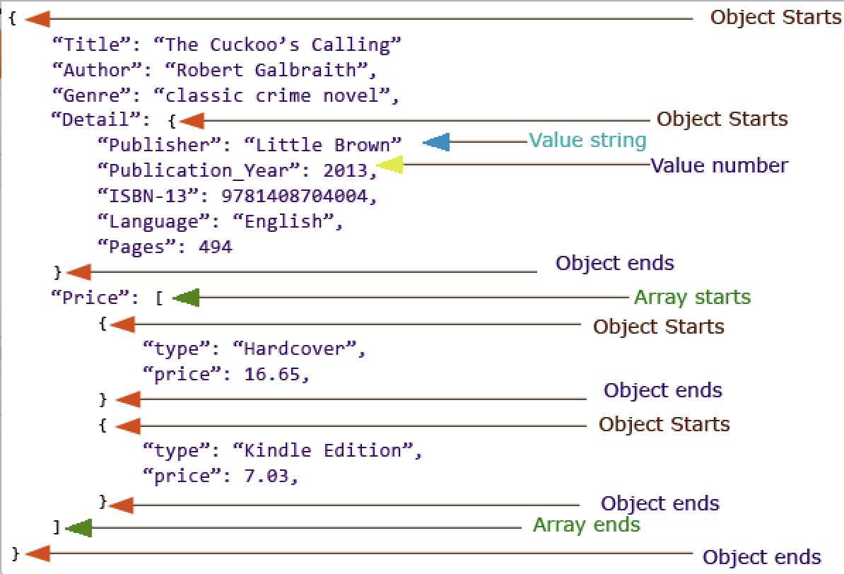
Intuitively, we can access data within the JSON object, such as
JSON.title="The Cuckoo's Calling"
JSON.Detail.Pages=494
JSON.Price[0].type="Hardcover"
Text-based Data-interchange Formats
Comma-separated values (CSV) and Tab-Separated Files are plain text files, where the first line is typically a header and the following lines are rows. These are typically in ASCII or plain text.
CSV Files
We can represent the same data as a CSV. The first row is typically the header.
newID,PC1,PC2,PC3,PC4
PPMI.Pilot.HA_ITG001_296597,0.108006766,0.015726028,0.093262438,0.060885093
PPMI.Pilot.HA_ITG002_PP0018.3690,0.104529423,0.017393778,0.117255688,0.07702544
PPMI.Pilot.HA_ITG003_PP0018.3682,0.107576826,0.002806186,0.171024597,0.071616656
PPMI.Pilot.HA_ITG004_3119622,0.074604492,0.049329752,-0.115794448,0.099060234
PPMI.Pilot.HA_ITG005_3145413,0.110742871,0.061465364,0.231489894,-0.070450761
PPMI.Pilot.HA_ITG006_953306,0.113388178,0.013073106,0.232587341,-0.002473437
PPMI.Pilot.HA_ITG007_1176618,0.065665593,0.080236696,-0.218573769,0.071228383
PPMI.Pilot.HA_ITG008_PP0015.9868,0.088975015,0.026523725,-0.02374357,0.10829439
There is a big problem here in that often “,” is used within documents. For this reason, csv is really not ideal. Some tools like R offer to use ” to help, but it’s still prone to problems. There are a few other issues, such as the use the unicode. More often than not, it’s best to have quotes (“) in them.
Another example of a CSV is below:

TSV (Tab Separated Files)
Tabs are /t in most tools such as Unix. In BASH you need to press control-v then press tab after letting go of control-v. We will use these a fair amount
newID PC1 PC2 PC3 PC4
PPMI.Pilot.HA_ITG001_296597 0.108006766 0.015726028 0.093262438 0.060885093PPMI.Pilot.HA_ITG001_296597 0.108006766 0.015726028 0.093262438 0.060885093
PPMI.Pilot.HA_ITG002_PP0018.3690 0.104529423 0.017393778 0.117255688 0.07702544PPMI.Pilot.HA_ITG002_PP0018.3690 0.104529423 0.017393778 0.117255688 0.07702544
PPMI.Pilot.HA_ITG003_PP0018.3682 0.107576826 0.002806186 0.171024597 0.071616656PPMI.Pilot.HA_ITG003_PP0018.3682 0.107576826 0.002806186 0.171024597 0.071616656
All of these are considered flat files. In the future, we will talk about structured tables and databases such as through SQL or PostGRSQL.
Aggregating, Pivoting, and Summarizing
One of the first major goals of understanding a dataset is to summarize it. Its easiest to think of in the context of table. For example, one may wish to know what the range or possible values/factors/categories is of a particular column, sorting by a given column, filtering it to remove certain rows, or perhaps create different ways of viewing that data by groupingit together. In part from the Excel nomenclature, this is referred to as pivoting or aggregating data.
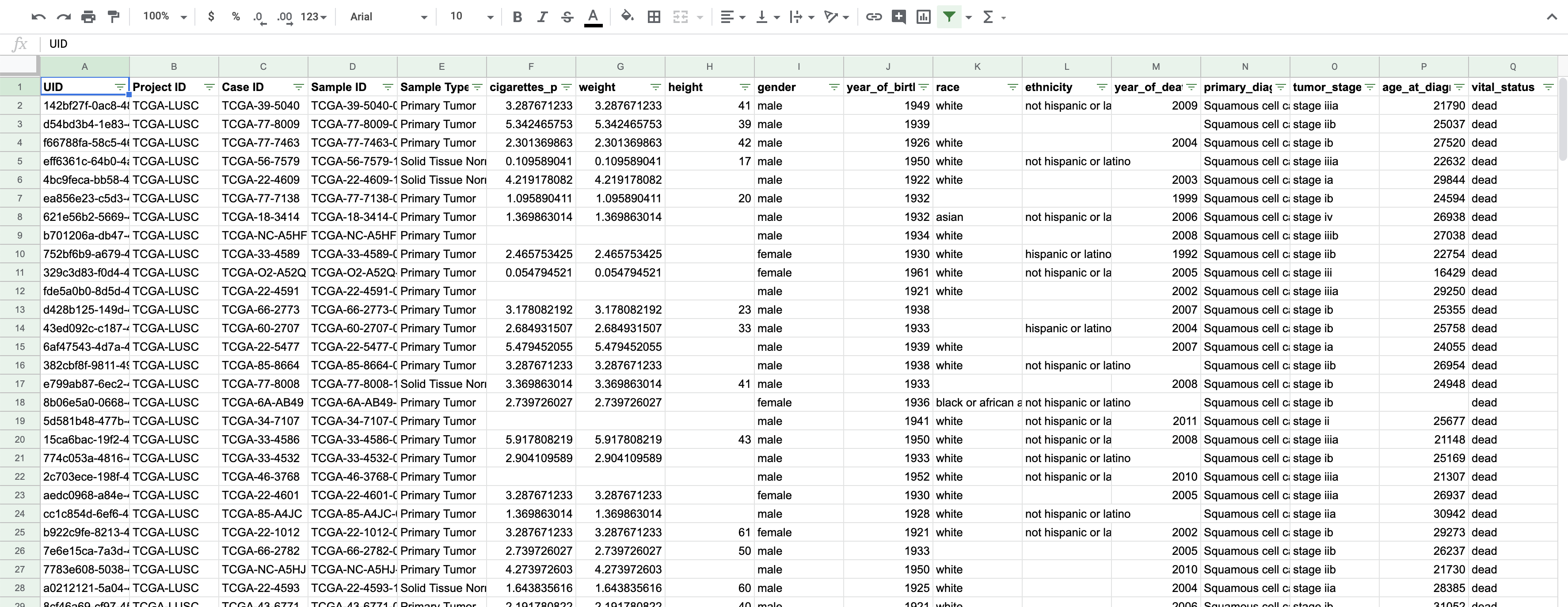
We can actually learn most of these using Google Sheets or Excel, though let’s use Google Sheets form the above data. I’ve gone already into the Data menu and selected create a filter. We will test out some of these ideas using a clinical sheet describing samples from within The Cancer Genome Atlas (TCGA), shown below. Later you can explore this dataset using the exercise link below.
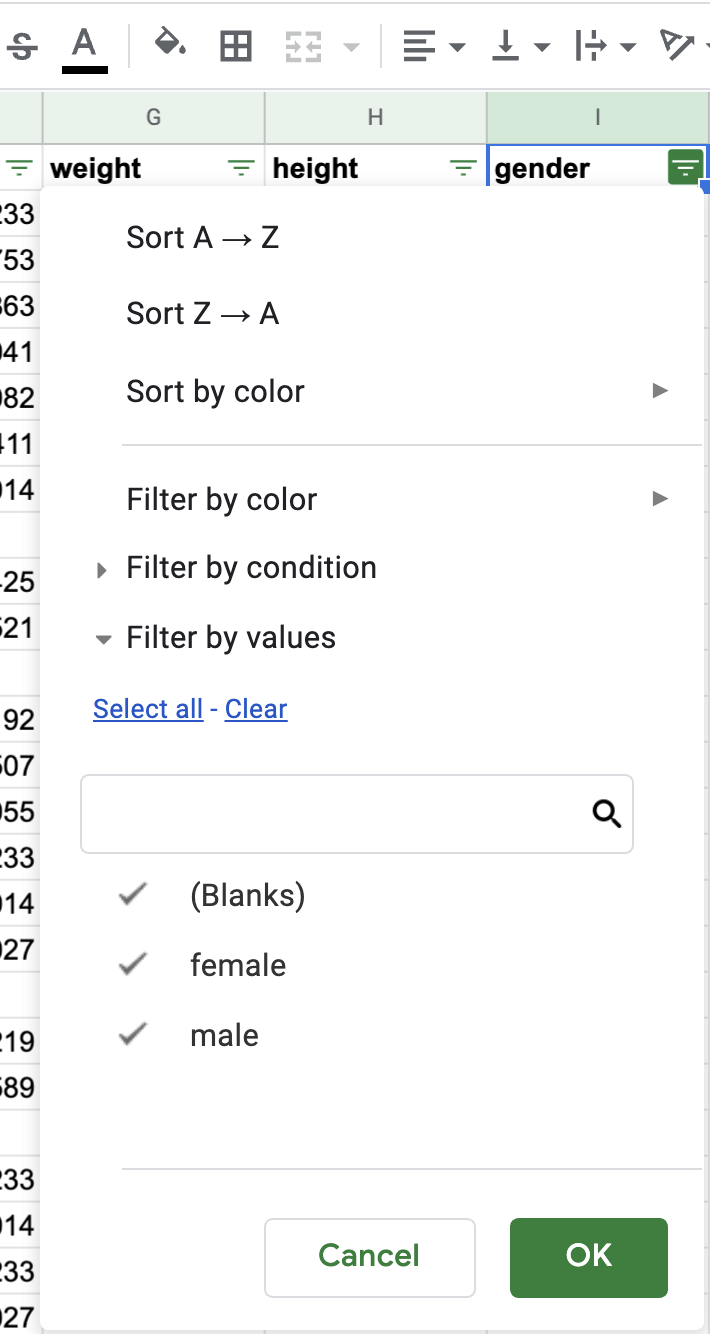
If we click on a header, we can see that we can both sort and add filters on the data. We can also see different categories of the data, such as the different genders.
Graphing Exercise
In the graphing exercise we below, start by clicking “load data”, or put in some tab/csv delimited data. As we change columns the applications changes to different types of graphs. Filtering gets interesting because we can effectively add complex conditions to our filtering, including using includes, greater than, and many other operations. We can join these together as well using and or or.
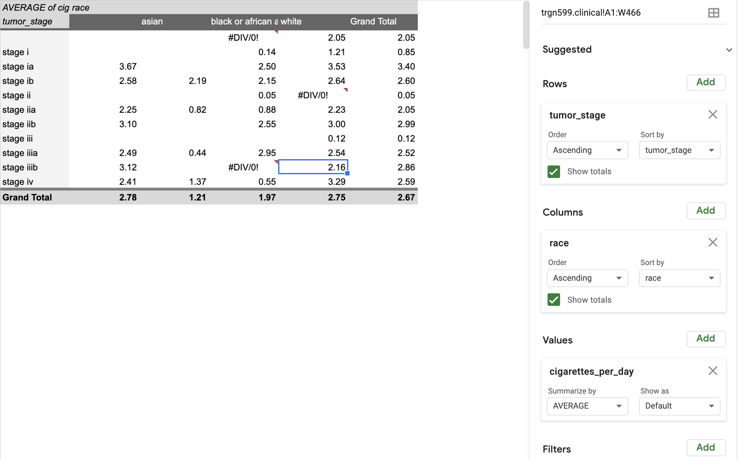
If we highlight all the data and click pivot table under the Data menu, we can do something really amazing, and create new tools that summarize the prior data by defining columns, rows, and fields of our new table.
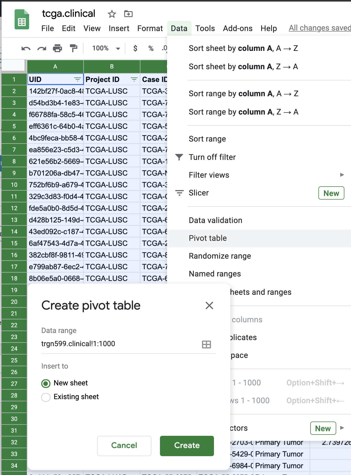
For example, we can count the number of times a certain group is found. We can do more than count, we can sum, take the mean, and many others. The key to do this is to identify which fields will be our new columns and rows, and what field will make up our values. Under the Pivot table editor in the right, click Add, then select the type of variable. Very important, we can count, and do many other operations as well. For example, we can example individuals who are part of the Tumor Cancer Genome Atlas (TCGA), and create a new graph of Average Number of Cigarettes per Day by Race, by adding rows and columns appropriately.
Exercises
Exercise 1:
Make a copy of the breast cancer TCGA Breast Cancer Data. Using the pivot functions, explore different aggregations of the data.
Exercise 2:
Download a table of TCGA Breast Cancer Clinical data:
Open this data in a text viewer. Look at the data by scrolling up and down. Now, paste the data into the text window below. Change the x-axis and explore different parameters to see how graphs for different types of data.