Understanding the Types of Data
It’s important to start with the idea that we have different data types. Data can be numbers, letters, dates, and so forth. Within a computer, these are all represented differently and in very defined ways.
What’s the difference between the number 2, the character 2, two, 2.0, 200%? Quite a bit, and the impact is significant to scientific data and data analysis. Recently, there was an article:
How can this arise? Open Excel and type the gene SEPT6and save it as a csv. For example, if we take a file and put:
Gene, Value
KRAS, 2.323
SEPT6, 2321
TP53, 2.1.2
Then we open it in excel and see that the data has changed. This can have far-reaching effects and is something to be careful:
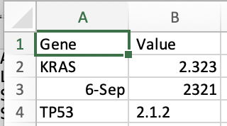
We then save it, and looking at the raw data, we see that the underlying data has changed.
Gene, Value
KRAS,2.323
6-Sep,2321
TP53, 2.1.2
What’s happening is that Excel is interpreting and determining the type of data and decides that SEPT6 should be a date. In Excel, date is a type of data. Accordingly, it then stores it in a way whereby fundamentally, it’s changed. Excel is a weak typing language and guesses what type of data is underlying. Other languages are strong typed. What does this mean, and what are some fundamental types? We review a few, but it’s important to understand each language types and these are some of the most primordial parts of data science we need to understand.
This video introduces the data topic in more detail, and we will cover its material in the next couple of weeks.
Written, Visual, and Applied Learning
The goal is to learn (1) first through listening to a screencast, (2) by reading the short vignettes used for the screencast, and (3) by exploring the interactive sessions either on the web page or via the JupyterLabs & Notebooks. The recommended way to use this resource is on the desktop using Google Chrome or Safari.
Written Content
Content and exercise are first provided as written HTML, viewable on any web browser by clicking on any of the above links. Controlled vocabulary or terms or highlighted, external sources are hyperlinked, code to use within Jupyter is shown boxed:
data=5
print("data is ",data)
The output is shown in gray boxes:
data is 5
Screencasts
Screencasts are available reviewing the written content and working within the Jupyter Labs/Notebooks.
Jupyter Labs & R Studio
These modules do not require you to have a Linux/Unix-based computer or have certain programs installed. All learning is done within browsers that run an environment where you can run Python, R, Command-line, Jupyter Labs, R Studio, and Notebooks.
Learning Unix TRGN Server & Through Examples of Realy analysis.
We will complete several weeks of analyses in population genetics and RNA-seq analysis using an analysis server that is Linux. These will help tie together key statistical concepts taught in other parts of the courses.
Recommended Readings & Web Resources
At times to struggle and it’s expected that you attempt to solve and figure out issues at least 2 to 4 hours before querying others. This is when learning occurs. Remember – searching for answers on the web is how many people identify bugs. Googling an error is standard SOP. Most issues will be typos.
A few thoughts on quotes – we’ll return here:
“this” is not the same as “this” or ‘this’ or `that`. Copy paste causes issues.
Learning to be Agile: Waterfall vs. Agile
There has been a monumental change in software and data analysis, particularly for retrospective analysis.
Waterfall. waterfall model is a relatively linear sequential design approach for certain areas of engineering design. In software development, it tends to be among the less iterative and flexible approaches, as progress flows in largely one direction (“downwards” like a waterfall) through the phases of conception, initiation, analysis, design, construction, testing, deployment, and maintenance.
The waterfall development model originated in the manufacturing and construction industries, where the highly structured physical environments meant that design changes became prohibitively expensive much sooner in the development process. When first adopted for software development, there were no recognized alternatives for knowledge-based creative work.
Agile software development is based on an incremental, iterative approach. Instead of in-depth planning at the beginning of the project, Agile methodologies are open to changing requirements over time and encourage constant feedback from the end-users. Cross-functional teams work on iterations of a product over a period of time, and this work is organized into a backlog that is prioritized based on business or customer value. The goal of each iteration is to produce a working product. In Agile methodologies, leadership encourages teamwork, accountability, and face-to-face communication. Business stakeholders and developers must work together to align the product with customer needs and company goals. Agile refers to any process that aligns with the concepts of the Agile Manifesto. In February 2001, 17 software developers met in Utah to discuss lightweight development methods. They published the Manifesto for Agile Software Development, which covered how they found “better ways of developing software by doing it and helping others do it” and included four values and 12 principles.
Resources to Learn Outside
Learning Flavors of Unix and Command-line
UNIX is an operating system in the 60s and broadly refers to a set of programs that all work the same way at the command line. They have the same feel. They have the same philosophy of design. Ok, it’s a specific operating system owned by AT&T. However, these days, it refers to a program that all follows a common framework. There are many types of Unix – MacOSX, Linux, and Solaris. Each is a different set of codes owned by different companies or groups to get the Unix common framework. MacOSX is owned and developed by Apple. Solaris is owned by Sun and Oracle. Linux is open-source and built from a community led by Linus Torvalds, and was meant to work on x86 PCs. The x86 refers to a CPU architecture used across most personal computers today (both Mac and PC). If I log into a Unix machine in 1980, 1990, 2000, 2010, or 2017 – it will often feel and work the same.
- Kenneth Bradnam’s Command line Bootcamp (http://rik.smith-unna.com/command_line_bootcamp). Free one-page resource.
- Lynda.com
- Various modules dependent on need
- Code Academy (https://www.codecademy.com/). An excellent resource for learning without an account. Evaluated resources include Learn the Command-line, Website building, and Git. Can be tested for free, or utilizes a $19.95/mo fee
- Ryan’s tutorial (https://ryanstutorials.net/bash-scripting-tutorial/). Quick and easy w/ good instruction.
Introduction to the Command Line
A Comparison: Windows over 20 years
Windows has generally seen many different Graphical User Interfaces (or GUI’s) over the years. Generally, the advent of Windows and key innovation was to remove the need for shell-level computing. However, much scripting and the ability to manipulate, wrangle, edit, and work with text was lost. Bioinformatics needs these tools, generally found in the various flavors ‘nix. There are ways to get to a ‘nix environment within Windows, such as through Cygwin or other VM devices but we generally don’t discuss that in this material.
High-level: What is Unix/Linux/Bash/Command-line?
These terms are used loosely and do not reflect their technical meaning. If I said to you that this course teaches Windows, for example, something comes to mind for most. However, technically, Windows could be Windows 95,98,3.1, ME, XP, and so forth. Same here – just more extreme. Learning command-line is generally the same as learning BASH (the most common shell environment) and learning to use Linux/Unix computers for most beginners. Down the road, there are important distinctions, so to keep all of this accessible to new users, we will not go down these rabbit holes.
Unix, Linux, and Command-line For Bioinformaticians
This module was originally developed for the command line and is being ported to Jupyter. We still have command-line instructions; at some level, it’s good to see those since so many recipes presume the command line. That said, it should always be straightforward to adapt these to Jupyter.
UNIX is an operating system developed in the 60s and broadly refers to a set of programs that all work the same way at the command line. They have the same feel. They have the same philosophy of design. Ok, it’s a specific operating system owned by AT&T. However, these days it refers to programs that all follow a common framework. There are many types of Unix – MacOSX, Linux, and Solaris and each of those is essentially different sets of codes owned by different companies or groups to get the common Unix common framework. MacOSX is owned and developed by Apple. Solaris is owned by Sun and Oracle. Linux is open-source and built from a community led by Linus Torvalds and was meant to work on x86 PCs. The x86 refers to a CPU architecture used across most personal computers today (both Mac and PC). If I log into a Unix machine in 1980, 1990, 2000, 2010, or 2017 – it will often feel and work the same. By comparison, Windows is not Unix. Even if you go to the command line, everything is different and changed over the years.
Command-line shells
Command-line shells are started up from a terminal program. Every Mac computer has Terminal preloaded. Start that up, and you’ll see a prompt from the shell. The shell is a program that responds to you, and you can change its look and feel. Most people like the shell that is called bash. With Catalina, there is a recommendation of using zsh. However, 15 years ago, tcsh was more common. There are others like c-shell (csh) and ksh.
Bash is pretty handy in that things like up-arrow takes you to the previous command, and you can press ‘tab’ to autocomplete. Now the important thing is that when bash starts .bash_profile is executed for login shells, while .bashrc is executed for interactive non-login shells. We can store a lot of settings here. Settings for the shell are also called environmental variables. You can see examples, such as typing echo $HOME' where echo simply prints the variable. $PATH is really important because to run any program, you would need to know the path to its location.
There are many different resources for learning command lines on Linux/Unix-based systems. Typically, a user may need to know 20 to 40 commands, with cd, ls, less being common. We have provided a cheat sheet below, and we link to some provided by others. All the commands have many options, and one can learn about them by typing man [command], ( ‘man grep’ for example). However, most people just google Linux command options. It is important to know that there are thousands of Linux commands, but most people only remember a small subset specific to their field. Some example resources are:
- https://learncodethehardway.org/unix/bash_cheat_sheet.pdf
- https://files.fosswire.com/2007/08/fwunixref.pdf
- https://www.cheatography.com/davechild/cheat-sheets/linux-command-line/
Working on servers

Much of data science involves remotely logging into a computer. A remote computer intended for other individuals or computers to connect to through the internet is called a server. How do we find the computer? It will typically have an internet protocol (IP Address: 35.225.22.109), and frequently it will have registered an official name, such as datasciencebioinformatics.org, that points to this IP.
There are many ways servers can be reached. A server has ports that can be opened and allow people to access programs. HTTP and HTTPS are the most common on ports 80 and 443. It’s so common the port numbers are generally not even required, and typically one just needs to type HTTPS://datasciencebioinformatics.org. When you do, your computer contacts the domain name server (DNS) to learn the computer’s IP, and then requests data port 80 or 443. This port is typically controlled by a web-server program, such as Apache, that responds to requests, such as HTTPS://datasciencebioinformatics.org/index.html, and knows to retrieve text, scripts, or the appropriate information. Your web browser gets this as text and, within your computer, puts together the HTML it receives to create web pages with a familiar look and feel.
We can typically look at the instructions, termed HTML, by using view source in the menu of your web browser. In this course, we will utilize Google Chrome, which is generally recommended for accessing materials.

However, other ports are used for different types of connections. We are going to log in to computers and run programs, manage them, and conduct complex analyses using command line. As we will learn, this involves using ssh to log in to computers. Again, ssh is so common that typically you don’t need to specify its port, 22. These servers can often access other servers and have resources connected to them. There are a few critical concepts that determine if a computer or server is able to facilitate the task we need.
Core Computing Concepts
Here we have a few important concepts bioinformatics must know well, and we start by providing a key question driving why that concept matters.
(1) Compute nodes.
Example Question: How many computers and how many cores do they have?
(2) Bandwidth (i/o)
Example Questions: How long does it take to read and write data, particularly if lots of processors or writing and reading on shared storage? How do we get the data into the HPC system?
(3) Memory
Example Question: How much do we need to put into memory – surely, a 3 Gbyte human genome is difficult to put into 2Gb of memory.
(4) Storage.
Example Question: How much storage do we need – where is it, and how is it maintained and managed? Where do we put data before and after?
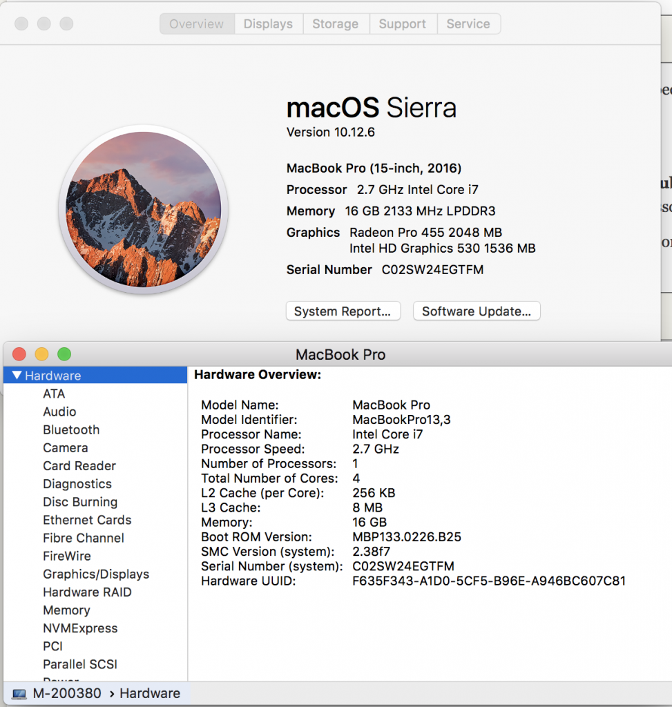
Lets learn about each of these by understanding your personal laptop. In the upper left hand corner of your screen, press the apple icon, and select “About this Mac”. We see information about processors, Memory, and Graphics. Let’s go deeper by clicking on System Report and looking at Hardware Overview.
Your laptop is like a compute node. We can see in the example below this laptop has an Intel Coreil at 2.7Ghz with one processor, and that processor has four cores. Each core can handle a thread. A thread would be, for example, a script (noting you can always spin off more processes within your script using &, and sending to background). We have 16 Gb of memory with 8Mb of L3 Cache and 256 of L2 Cache. These latter two are important, but the key for us is the 16 Gb. The more memory, the more things we can open at once – more windows, etc.
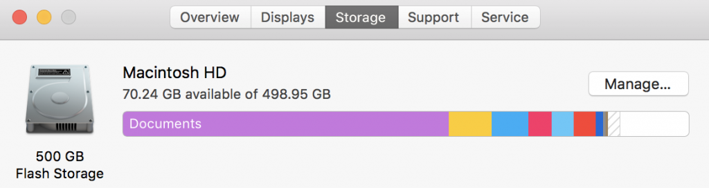
We can also click on storage from “About our Mac” to see how much storage we have and how much is used. Storage isn’t active – it’s like having a lot of music on a portal MP3 player – except MP3s take up a little bit of space. In this case, I have 500 Gb of flash storage. Flash storage is fixed and doesn’t involve a spinning disk – your new iPhone and your iPads are flashes, and the original large iPods were spinning disks. Spinning disks usually hold more – they also and always eventually break.
Accessing command line with Windows, Mac, and others.
Windows
Recommended: https://www.putty.org/
Native BASH in Windows: https://docs.microsoft.com/en-us/windows/wsl/install-win10
Macos:
Or just use “Terminal” already installed.
Development Environments Such As Jupyter
In a world where tasks must be completed in the quickest possible way, learning to code (the basics at least) is essential. But this just seems like a vast task and it’s difficult to figure out where to begin. Well, that’s what we’re hoping this series of modules will accomplish. They are essentially a gateway to introduce you to some introductory concepts in BASH, Python and R. You will be able to give it a go and write some code yourself, too!
Before we begin, there are some quick steps you must take to set things up. The modules rely on using two interactive development environments: Jupyter and RStudio.
The Bioinformatics Educational Module series uses two interactive development environments: Jupyter and RStudio. This webpage will walk you through setting up and running these environments successfully.
The JupyterLab environment provides multi-faceted functionality and, eventually, is where you want to go. We will use three major functions: Notebooks, Markdowns, and Terminal. We provide a link, and you can launch it within your web browser. It is also possible to install it on your local machine and conduct all your analysis within JupyterLabs. This is more of an advanced topic, so we presume you are using a web browser.
Overview
 The JupyterLab environment allows you to work on these different components together and have them displayed to you in a single window. We see a directory tree in the frame below with files, data, and code. We see a
 example notebooks with code that has been rendered. We see an example csv file with raw data. We see a markdown document as raw text and as the rendered version. We see a window with stand-alone python code that could primarily run within a notebook’s code blocks or by the command line. Lastly, we see a terminal command-line interface where BASH commands can be entered. 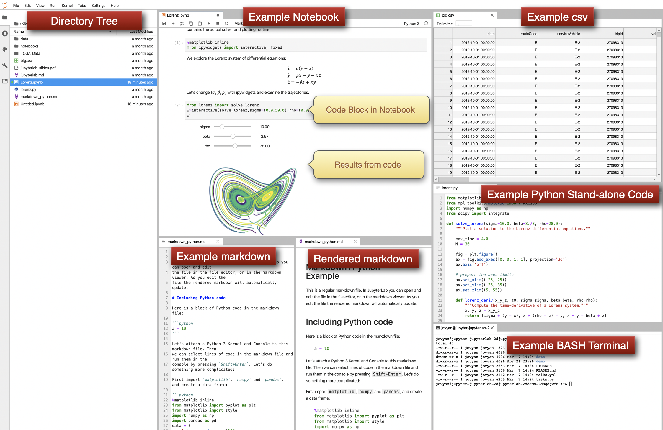
Markdowns
Markdown is is a lightweight markup language that is plain text formatted, but is rendered to look like a web-page. It has a way of creating code-blocks. For example on the left, we see Markdown. On the right, we see the rendered view that could be published 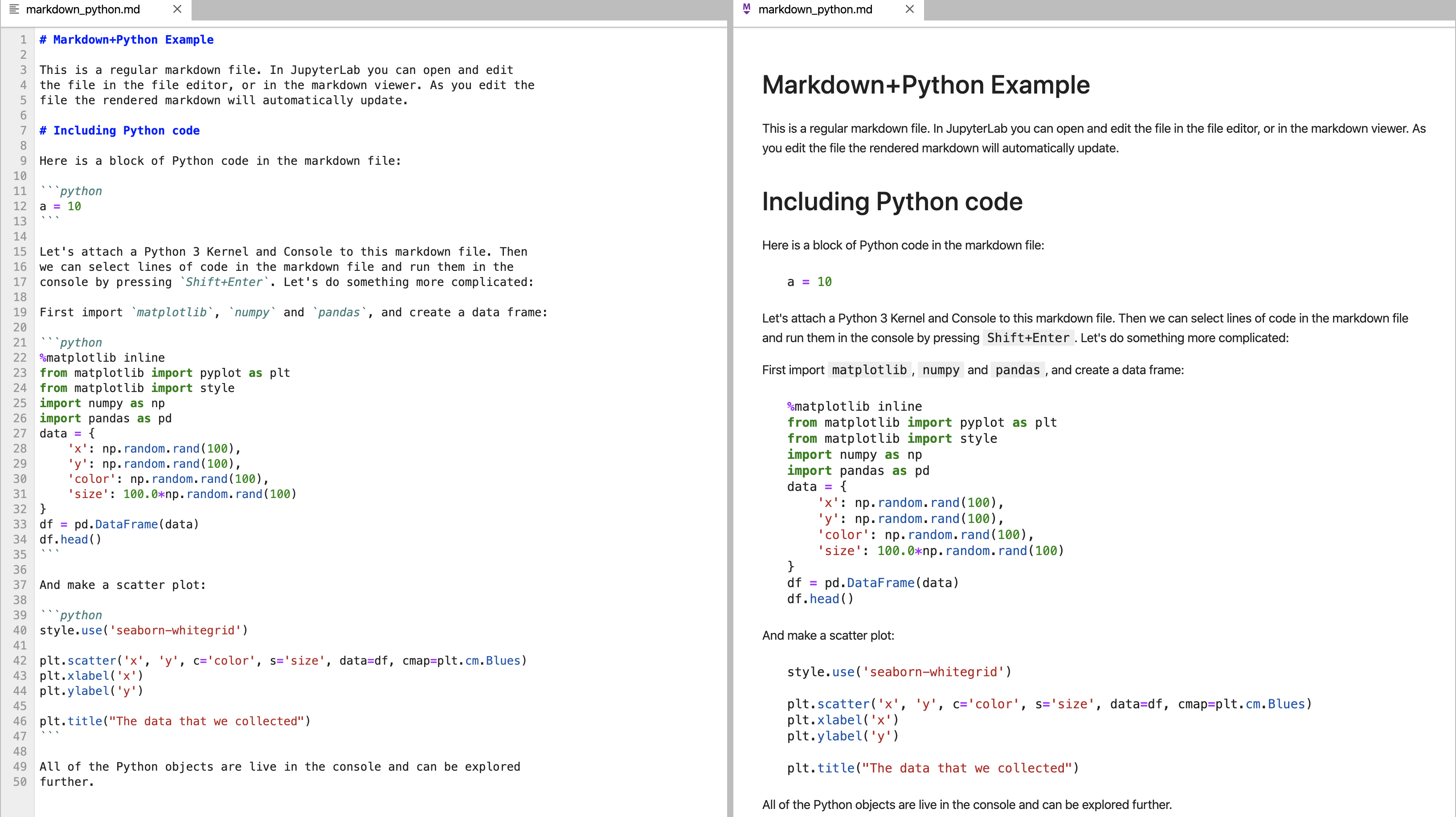
Jupyter Notebooks
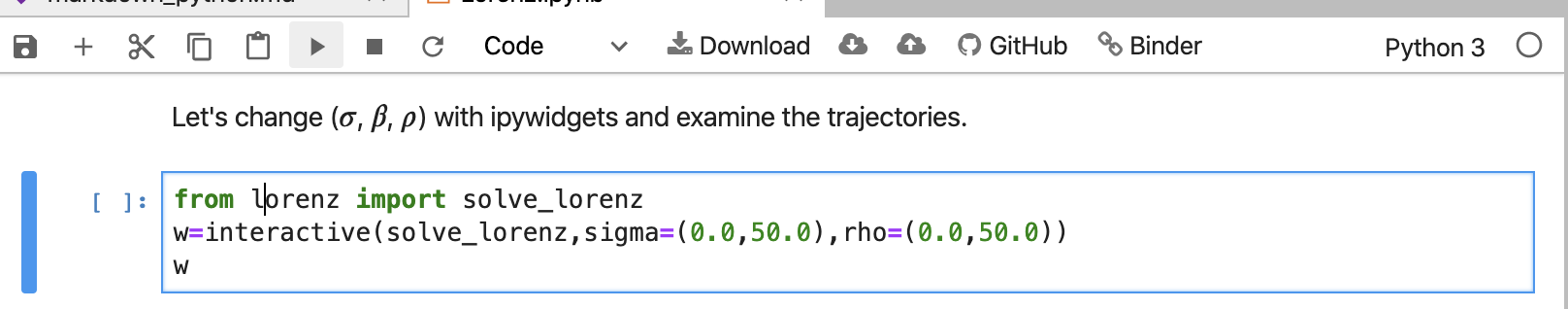
Think of Jupyter Notebooks like a lab notebook. Jupyter Notebooks is a way to create short python scripts, show their results, and have formatted commentary/text in a single document. Typically, one describes the analysis they are doing and then puts the code conducting analysis in sections called codeblocks. Results such as graphs appear below the code after it has rendered. 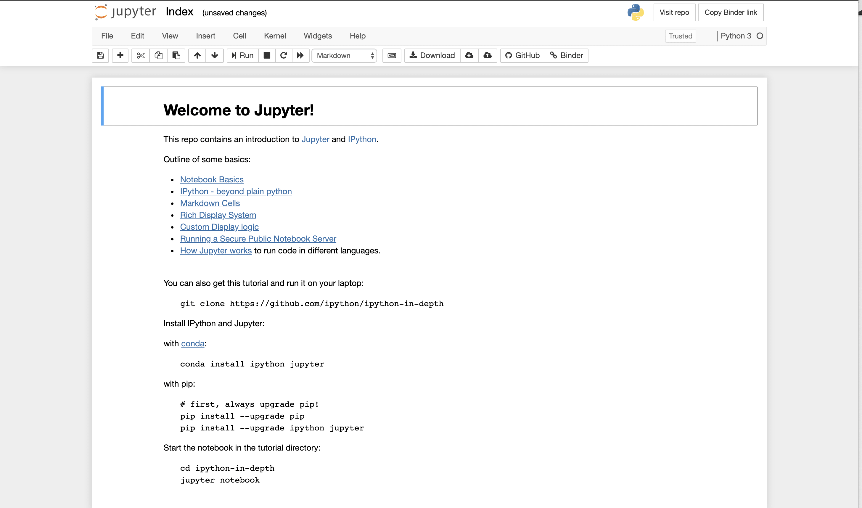 In many parts of the tutorial, we just use the notebook that is described below. However, if you want full functionality and saving, you do want to move to install locally JupyterLab. There is a version that can be run within your browser. https://jupyter.org/try A snapshot is shown below. You can see in this view, you can see all files, you can edit and create what is called
 markdowns in the middle frame, and you have rendered markdowns in the right frame. We have discussed markdowns before, but basically they are a way of putting code and text together in a way that looks like a web page. The code is run in cells by pressing the forward arrow after clicking on the cell.
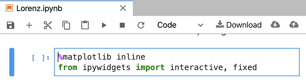
Code blocks are magical cells – creating interactive computing.
Now those code blocks are a bit magical in Jupyter lab as you’ll see. You’ll be edit and run them, seeing the results in a live interactive view. These types of markdowns that expect to be run and create a reproducible analysis are actually notebooks, and in Juptyer labs they end in .pynb. Notice that I can actually hit play or ‘run’ and see code by analyzed.There is quite a bit to learn and to make the materials accessible, we only touch the surface. I encourage you to learn more about Jupyter Labs, Notebooks, and so forth. It’s an amazing data science vehicle – and also a great learning tool.
Getting Started
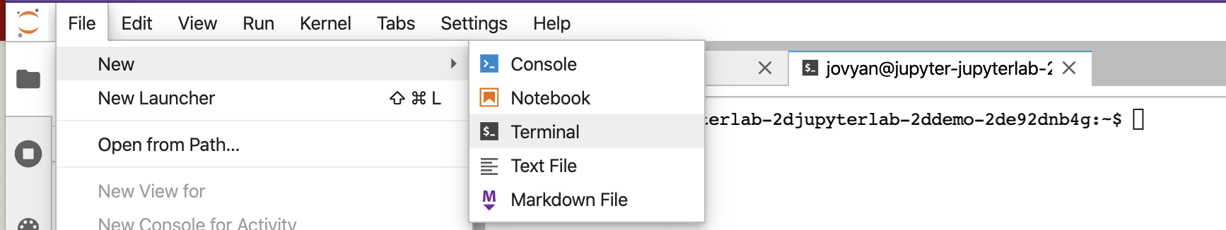
We will use the console part of JupyterLabs for this section. You’ll want to start in a new window.
This module is meant to be a broad and very basic introduction to the command line and you will learn enough to be functional. We have modules where we provide more detail, but they require a Unix-based computer (like Mac), and this module leverages a web interface: Jupyter Labs. This is done because many users will be on Windows-based machines and may not have access to a Unix-Linux based computer. Begin by opening a new JupyterLab window and navigating to the terminal option from the dropdown.
You would see something similar to the below.
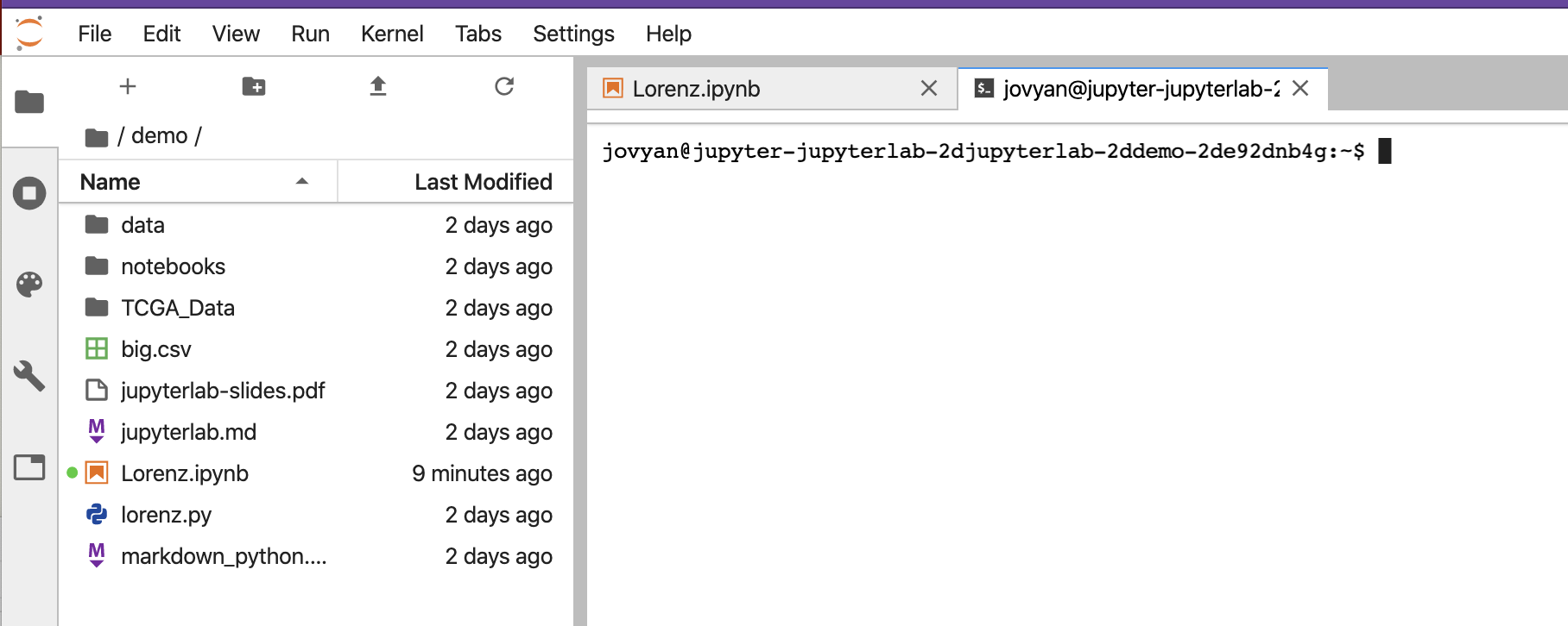
On the left above is a file structure with several starter files in it. On the right is the terminal that we will use as our learning environment.
Videos