History

The Dryden Wind Tunnel has an illustrious history. Here follows a brief* illustrated view through some of the highlights.  This is far from a complete story, but selected references are given, from which a detailed map of the exciting developments in fluid mechanics, associated with this wind tunnel in particular, can be drawn.

• maybe not so brief. To enjoy the story, you probably need to set aside 15 minutes or so.

Early 1900’s and the mystery of turbulence

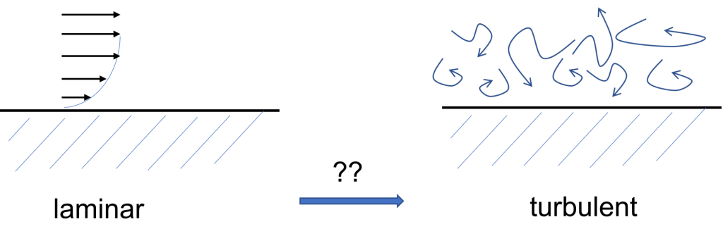
In the early 1900’s the science, engineering and mathematical study of aerodynamics was just beginning, amidst tension between mathematical and theoretical studies and more applied and practical concerns. In 1904 Prandtl [Pr04] had introduced his famous and powerful boundary layer theory of viscous fluid flows. There was a practical realization that these smooth and predictable (and mathematically tractable) profiles could be disrupted and the ensuing turbulent flow was both complex and likely the cause of significant deterioration in performance of bodies such as airfoils and wings.  The problem is shown in cartoon in Fig. 1.

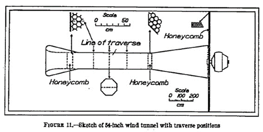
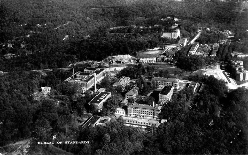
Over the period 1909 — 1918, a number of wind tunnels were in operation around the world (see Fig. 2) but there were difficulties in reconciling different results from seemingly similar configurations. In 1920, Hugh Dryden in NBS paper# 394 [Dr20] entitled “Air Forces on Circular Cylinders, Axes Normal to the Wind, with Special Reference to Dynamical Similarity.” tackled the two principal problems facing the community. They were: (1) Under what circumstances could the imperfect flow of a wind tunnel be expected to present a realistic medium for tests designed for free flight in air? (2) When and how could necessarily smaller scale model tests be extrapolated out to real wings and aircraft?

There was a growing awareness that the background turbulence mattered, both in wind tunnels and in real applications. Now the community needed to understand and characterize turbulence, find ways of indicating its magnitude, and develop tests to demonstrate that. This required the development of new and more sensitive instrumentation.

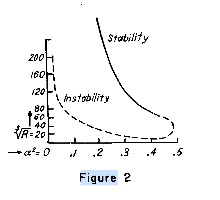
Meanwhile, theoretical work was underway, and Arnold Sommerfeld guided the PhD theses of two specially promising students. The first was Werner Heisenberg who in 1924 published his thesis [He24] demonstrating that, seemingly paradoxically, viscosity could destabilise a laminar flow and that profiles existed that were capable of undamped oscillations at some finite (but large) value of the Reynolds number, R. (Heisenberg suggested that a real Reynolds number as it appears in the equations should be aR, the product of initial growth rate, a, times R.) The mathematics were formidable and were the first efforts to solve what are now known as the Orr-Sommerfeld equations. Though undamped oscillations were shown to be possible, it was not demonstrated at what critical R, even though a qualitative stability diagram indeed appeared in roughly the same form as would later become familiar (Fig. 3).

In the year he produced his thesis, he attended a series of lectures by Neils Bohr, coming under the spell of quantum mechanics. Two years later he would publish his seminal work on the subject. Meanwhile, Tollmien worked on the same problem and in 1929 [To29] showed a class of instabilities in the laminar boundary that could grow at a certain critical R, providing the seeds for generation of turbulence in wall-bounded flows.

These two dimensional wave solutions, subsequently known as Tollmien-Schlichting (T-S) waves [To29, Sc29] were elegant and predictive, and invisible: that is to say no-one had been able to detect such objects. Did they not exist? Or could current techniques simply not find them?

1920 – 1937 The development of the modern wind tunnel

Dryden and colleagues set about understanding and reducing wind tunnel turbulence.  A report NBS#321 by Dryden & Heald in 1926 [Dr26] began to systematically investigate turbulence in the wind tunnel.  Their summary can be quoted in full:

“Two methods of making studies of turbulence are described in this report, together with the results of their use in the 54-inch wind tunnel of the Bureau of Standards. The first method consists in measuring the drag of circular cylinders; the second, in measuring the static pressure at some fixed point. Both methods show that the flow is not entirely free from irregularities.

We have shown that the main fluctuations of static pressure in our 54-inch wind tunnel are associated with the unequal driving force over the tunnel mouth. There is a pattern of static pressure changes accompanying the propeller in its revolution. We have pointed out the difficulties encountered in attempting to make measurements by means of a Pitot tube connected to a sensitive gauge.”

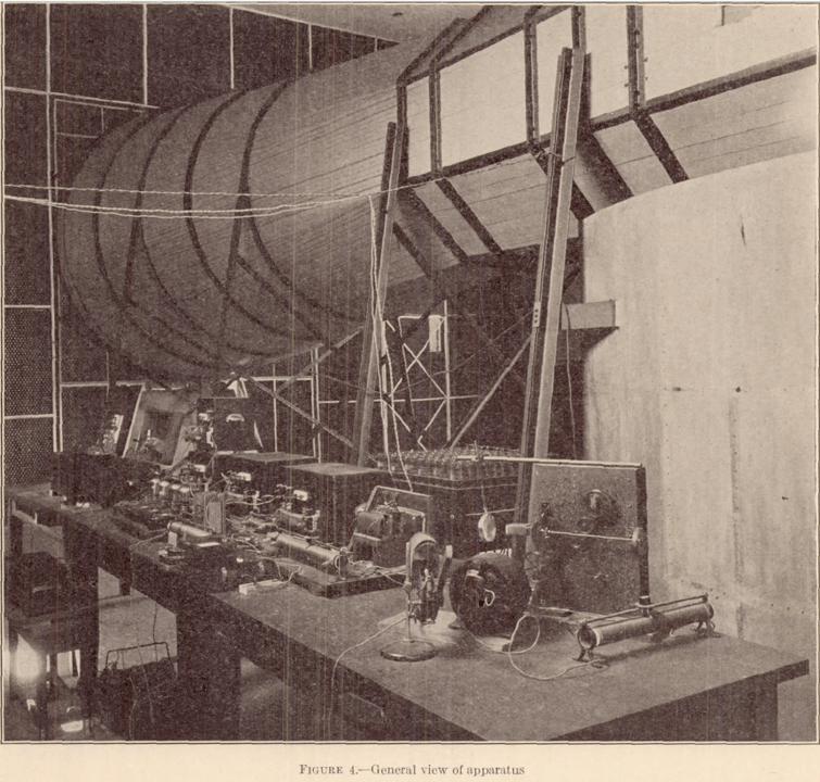
These ideas and insufficiency of the Pitot tube led to the accelerated development of hot-wire anemometry, where the cooling rate of a heated wire is used to deduce the convective flow speed over that wire.  In practice the wire is held at a constant temperature and the current fluctuations required to do this are related to the flow speed.  The application of this device to turbulent flows was a very demanding extrapolation and Dryden and Kuethe in 1929 [Dr29] wrote an authoritative work on how the whole apparatus performed.  The authors concluded;

“The apparatus described is very bulky, far from portable, and in many respects inconvenient to use. We believe, however, that a great improvement is possible, …” 

Fig. 5 gives an idea of the scale of the equipment involved.  Almost 100 years later, the hot wire remains the standard for high-frequency measurement of fluctuating velocities in air.

We can see that the authors necessarily concerned themselves not only with the tunnel properties but also with the instrumentation available for its measure.  First, it was obvious that wind tunnel design and methodology needed revisiting in order to characterize, control and reduce the background turbulence.

One of the main devices for doing this was by forcing the flow through screens composed of fine mesh wires.  But what type of screens worked best?  A series of tests was conducted, appearing in NBS Report# 581 [Dr36] (fig. 6)

The introduction concisely describes the current unsatisfactory state:

“The turbulence of the air stream is generally recognized as a variable of considerable importance in many aerodynamic phenomena, especially those observed in wind tunnels. The drag of an airship model may vary by a factor of 2, the drag of a sphere by a factor of 4, and the maximum lift of an airfoil by a factor of 1.3 in air streams of different turbulence.”

There were two significant advances in the 1936 report.  The first was a recognition that the characteristic length scales of turbulence need consideration – not all turbulence was the same in altering separation and drag characteristics.  Dryden et al. used a pair of hot wires, separated by a variable distance, and could then form a correlation function for the two signals.  The correlation function described not only the spatial characteristics of the turbulence behind various screen geometries, but also allowed corrections to the hot-wire signals themselves when the turbulence scales reach down to the scales of the wire.

The authors took up themes from G.I. Taylor’s recent work on the fluid dynamics of turbulence and considered in detail how such flows would decay in a tunnel environment.  The critical Reynolds number for flow transition over a sphere had been used as a proxy for turbulence measurement but without good agreement between different facilities, or even different-sized spheres.  Finding that the turbulence scale relative to the sphere size was important, the authors also considered how turbulence would affect the aerodynamics of other bodies, such as wings.

A number of points were emerging.  Screens could be used to create small-scale turbulence, whose decay would then be associated with reduced amplitude turbulence downstream (Fig. 7).  Tunnel design should account for the whole path taken by the fluid as it travels through the test section and then eventually back to the drive fan, whose mechanical properties were also influential.  Certain aspects of the instrumentation could be significantly improved, and the finite-time response of hot-wire devices was a concern.

1938 and the war years – the new wind tunnel at NBS

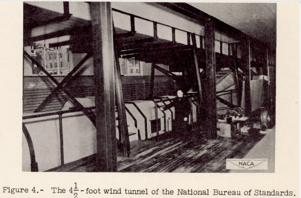
Advances in tunnel design and instrumentation thus occurred in concert, and in the following year, 1938, a very new wind tunnel configuration had been completed, shepherded by Dryden (Fig. 8).

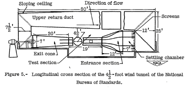
In the late 1930’s relations between German and US and British engineers were strained and numerous developments were classified as secret, delaying (or preventing) publications for years to come.  The redeveloped wind tunnel plans were eventually made public in a 1948 NACA TN 1755 [Dr48].  Note the appearance of the National Advisory Committee for Aeronautics, and this publication as a Technical Note.  The NACA TN literature has been an extraordinary resource for science and engineering in aeronautics.

Fig. 8 shows the tunnel design which stands today.  The flow is closed-circuit, with gradually sloping walls to manage the pressure gradients and wall boundary layers, turning vanes guided the recirculating flow around the low-speed corners (the flow is clockwise in Fig. 7).  A number of turbulence screens are arranged at the beginning of the settling chamber, well before a contraction section which is quite gentle and modest by today’s standard, Asettle:Atest = 12/4.5 = 2.67.  The single remaining element from the old design is the size and shape of the test section itself: an octagon of 4 ½ ft (1.37 m) face-to-face dimension.

T-S waves and boundary-layer transition

Again, it is informative to read the summary/abstract of the NACA TN 1755 paper verbatim:

“Within the past 10 years there have been placed in operation in the United States four low-turbulence wind tunnels of moderate cross-sectional area and speed, one at the National Bureau of Standards, two at the NACA Langley Laboratory, and one at the NACA Ames Laboratory.  In these wind tunnels the magnitude of the turbulent velocity fluctuations is of the order of 0.0001 to 0.001 times the mean velocity.The existence of these wind tunnels has made possible the development of low-drag wing sections and the experimental demonstration of the unstable laminar boundary-layer oscillations predicted many years ago by a theory formulated by Tollmien and Schlichting.

The development of the low-turbulence wind tunnels was greatly dependent on the development of the hot-wire anemometer for turbulence measurements, measurements of the decay of turbulence behind screens, measurements of the effect of damping screens on wind-tunnel turbulence, measurements of the flow near a flat plate in air streams of varying turbulence, and measurements of the drag of specially designed low-drag airfoils. These investigations were conducted in collaboration with Schubauer, Skramstad, Jacobs, Von Doenhoff and other members of the staff of the National Bureau of Standards and the National Advisory Committee for Aeronautics , Von Karman and Liepmann of the California Institute of Technology, and G. T. Taylor and his colleagues at Cambridge University.

This paper reviews briefly the state of knowledge in these various fields and those features of the results which make possible the attainment of low turbulence in wind tunnels. Specific applications to two wind tunnels are described.”

The summary describes an international collaboration and systematic nationwide effort in the US to design and characterize wind tunnels for accurate prediction and measurement of aeronautical quantities.  The lowest turbulence levels of 0.01% were remarkable, and sufficient so that the long-predicted T-S waves were finally revealed.  The person most responsible for the new NBS tunnel was Hugh Dryden, shown next to his creation in Fig. 9.

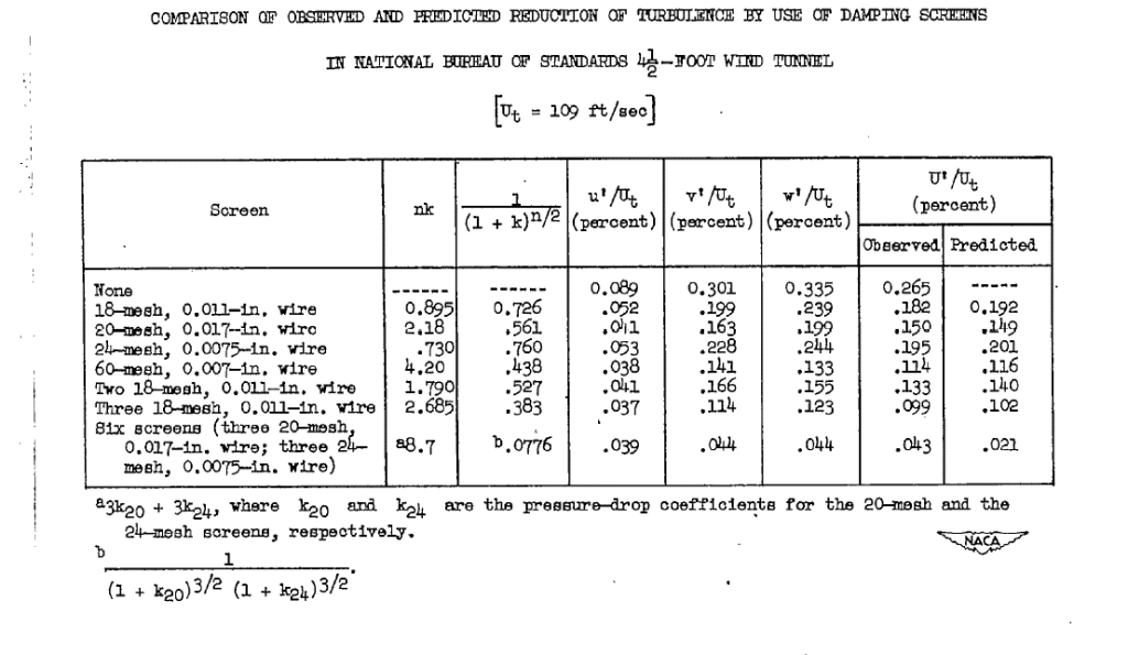
The tunnel and instrumentation methods were meticulously analysed and documented.  Fig. 10 shows an important table of the measured turbulence characteristics behind varying screen geometries, with the last line being a combination of previous types.  A further publication devoted to the properties of damping screens was published by Schubauer, Spangenberg & Klebanoff as NACA TN 2001 in 1950 [Sc50].  In the introduction we read that the study itself was promoted by Dryden and GI Taylor.

Galen Schubauer at NBS had worked tirelessly for many years towards understanding and measuring flow instabilities in transition.  This work was sometimes funded, sometimes not.  Sometimes he was encouraged by Dryden (now head of the Aerodynamics Section at NBS), sometimes not.  When the two finally did collaborate to secure funding, the work was classified as Confidential.  The first open literature paper on natural transition in laminar boundary layers was by Schubauer & Skramstad [Sc47] (A prior 1946 report by Schubauer and Klebanoff [Sc46] was classified.)

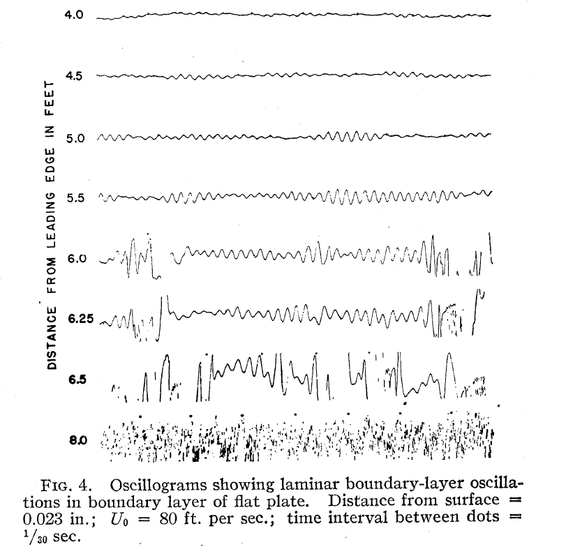
Fig. 11 shows the first demonstration of T-S waves, which the authors termed ‘boundary-layer oscillations’.  The amplitude and wavelength of the boundary layer oscillations was in good agreement with the theoretical works of Tollmien and Schlichting (who worked independently), and Schubauer and Skramstad noted “The general applicability of the theories of Tollmein (sic.), Schlichting, and Lin can no longer be doubted.” 

Schubauer and Skramstad measured the frequencies of naturally-occurring waves such as seen in Fig. 11 and compared them with theoretical predictions (Fig. 12).  The agreement of observations with predicted most amplified frequencies is good.  One point denoted by a cross in Fig. 12 was measurable for artificially elevated background turbulence levels and it too lies close to the stability boundary.  It was the only such point measurable and the authors noted how the similar turbulence levels in all other tunnels would have rendered these observations impossible.  We now understand these other phenomena as by-pass transition where ambient disturbances of sufficient magnitude cause a direct transition to turbulence without passing through the T-S wave.

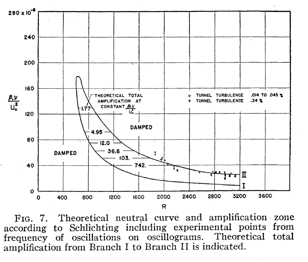
Schubauer and Skramstad further conducted experiments in forcing the disturbances at known frequencies, first through global and then local acoustic excitation, and then finally with a vibrating ribbon.  The ribbon could excite a range of frequencies that traversed the damped-neutral-amplified-neutral-damped boundaries in R (which increases with x) and the agreement between experiment and theory (Fig. 13) for the neutral curves is very good.

The existence of T-S waves in a developing boundary layer was definitively confirmed, as was their central role in determining transition to turbulence.

1950’s

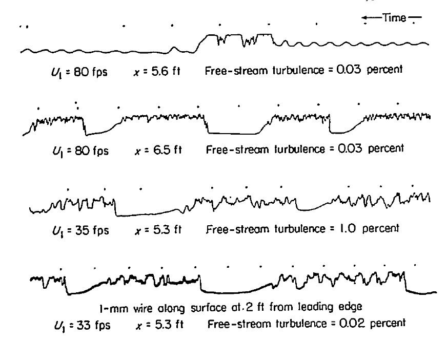
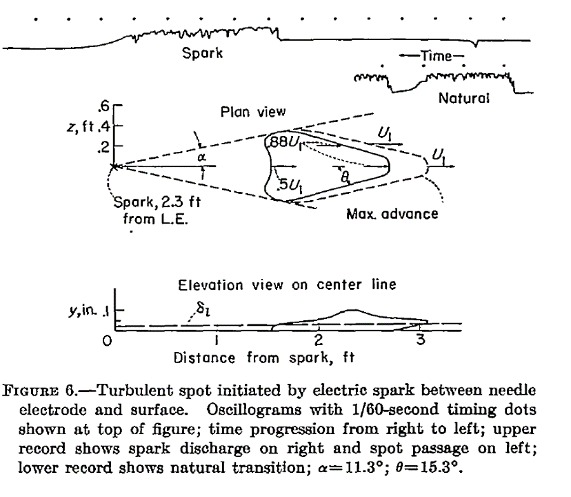
In 1955 Schubauer & Klebanoff [Sc55] published an account of the development of natural and forced transition in a laminar boundary-layer.  In particular, they noted the intermittency of the first transitional spots, and the calm period that lay behind them, where turbulence could not be provoked (Fig. 14).  The study also showed that the turbulent spot could be triggered by a local spark discharge so a picture could be built up of the spatial structure of the turbulent spot (Fig. 15).

Experiments continued in the NBS wind tunnel throughout the 1950’s, where its low turbulence levels made it uniquely suited to transition and turbulence studies without confounding facility effects. Klebanoff was a key figure in many of these studies.  In [Kl55] he studied the turbulent boundary layer in the context of the now more-widely understood statistical theory of turbulence, which appeared to apply well for isotropic turbulence.  Wall-bounded shear flow is not isotropic, so presents some formidable problems in analysis.  It was found that near the wall, where most kinetic energy dissipation occurs, concepts based on isotropy were inadequate.  One J. Laufer was recognized in the paper for ‘stimulating discussions’ and he was also cited for important studies of turbulence in channel and pipe flow [La51, La54].  John Laufer in 1964 was the founding member of the USC Department of Aerospace Engineering, and it was he who would arrange for the transfer of the NBS wind tunnel to USC.

The NBS wind tunnel was by now well-established as a powerful apparatus for the study of many fluid dynamical phenomena, and work continued with Klebanoff and others through into the early 1970’s.

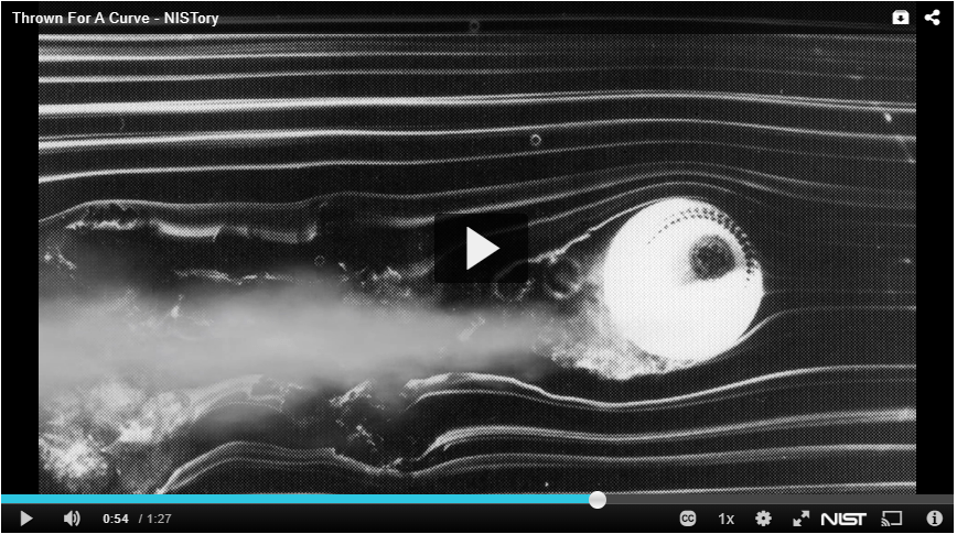
As a footnote to the 1950’s we may add the curious study of the spin of the baseball.  Lyman Briggs was the former director of NBS and in 1959 he enlisted the assistance of the NBS wind tunnel and 2 pitchers from the Washington Senators to resolve the question of whether a baseball could truly curve in its trajectory.  Apparently this matter was still open to debate, some arguing that the appearance of curvature was an optical illusion.

Those involved were also apparently unaware of the demonstration of side-force due to spin by Magnus in 1853 [Ma53], and of the mathematical analysis by Rayleigh in 1877 [Ra77], where the targets were missiles and tennis balls, respectively.  The solution by Rayleigh was in fact a critical step in the attempts for an aerodynamic explanation of lift in a frictionless fluid, and the circulatory component due to spin mirrored the much-neglected circulatory theory of lift developed by Lanchester [La07]. Briggs [Br59] published the results for induced curvature of both smooth and seamed balls, and the title includes a reference to Magnus’ paper, but the results were treated as entirely new.

Sports in the US often seem to operate by their own unique rules so it is not inexplicable that a new demonstration/solution was expected, and also that it be done in a practical device.  The baseball was spun on the axis of a vertical rod and side-forces were measured, the rotation rate being given by the winding of a trailing ribbon. Indeed it was verified that over its usual 18.4 m flight, a baseball could deviate due to spin by up to 44 cm (or 2 — 3 %).

1960’s onwards

The appearance of turbulent spots, such as those shown in Fig. 15, is a sign that not all the mechanics of boundary layer transition can be explained through purely two-dimensional instability waves.  Though the initial amplification of the T-S modes had been demonstrated beyond doubt in data such as Figs 11-13, the subsequent development stages appeared to involve amplification of three-dimensional motions, and then a third stage where nonlinear effects rapidly transition into turbulence.

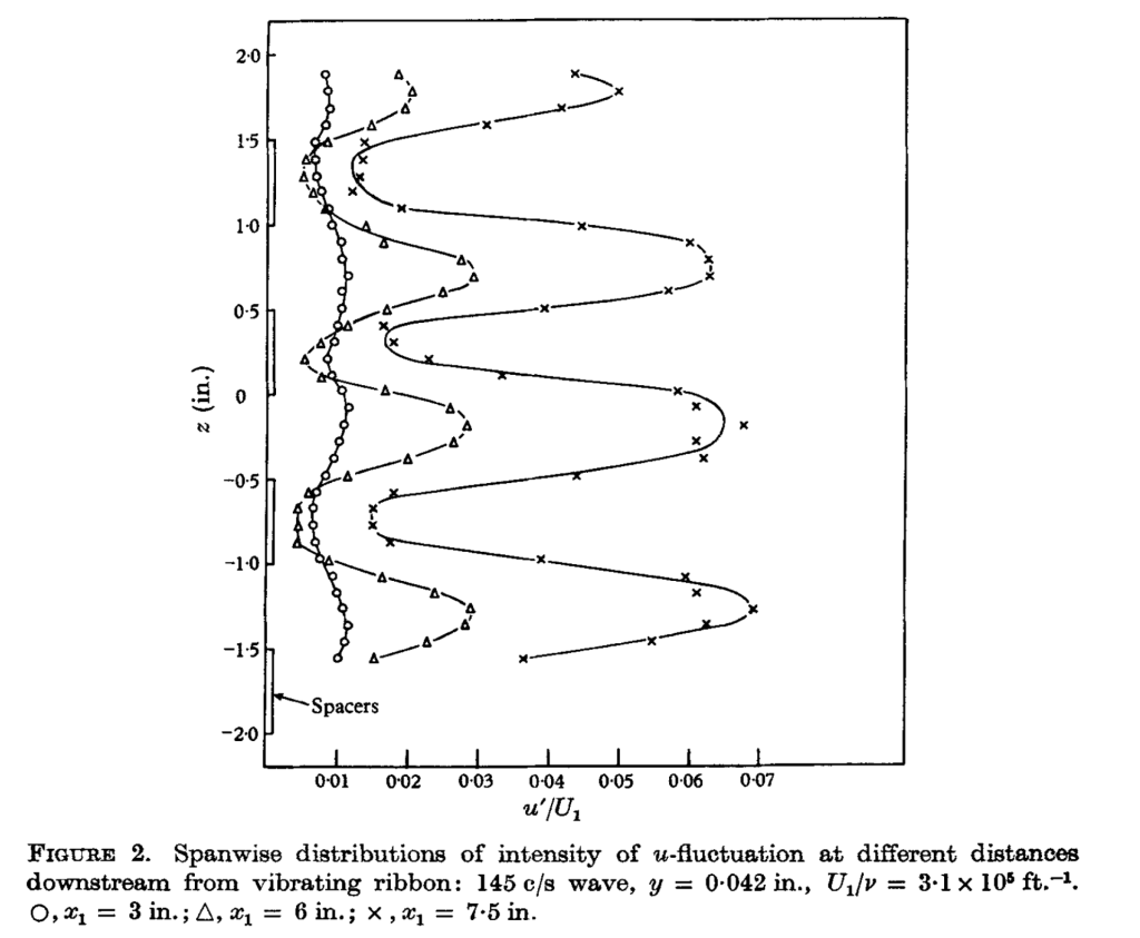
In 1962 Klebanoff [Kl62] published a study on the later stages of development, again using the vibrating ribbon mechanism to force the transition.  To properly control/study the three-dimensional modes, it was very important not only that turbulence levels were low but also that three-dimensional variations in the oncoming freestream be as low as possible.  The NBS wind tunnel was improved again through insertion of extra screens to make this the case.  The investigation could now focus directly on the flow speeds and locations where it was known that maximum T-S amplitudes would be observed.  The ribbon vibration itself was modulated in the spanwise direction to control the location of three-dimensional modes, which are shown in Fig. 17.

The 3D modes were associated with a system of longitudinal vortices and there was some discussion about whether these longitudinal (or streamwise) vortices were part of a collection of vortex loops (as had been noticed in some water-channel dye visualizations) and were termed here hairpin eddies.  Regardless, it was also noted that the final stage of very rapid growth and breakdown of the flow must involve nonlinear mechanisms that were still only partially recognized and understood.

Finally, in addition to the technical content, we may also see the diffusion of research now from government-sponsored technical labs and reports into international journals, such as the Journal of Fluid Mechanics (itself founded in 1956).

The study of three-dimensional instability modes and the control of transition continued into the 1960’s and beyond.  Klebanoff and Tidstrom [Kl72] described a study of the flow behind a roughness element (they used a two dimensional one) to show that the roughness elements work by generating an unstable boundary layer profile.  A consequence of this observation is that the shape of a roughness element could be influential.

As the fluids community wrestled with the questions of whether isotropic turbulence and its associated closure schemes were based on reality, there were numerous studies that deliberately attempted to construct homogeneous, isotropic turbulence, for example behind grids of various kinds.  Frenkiel and Klebanoff [Fr67] applied a rigorous analysis of hot-wire signals and their correlations and calibrations to show that higher order statistics (third-order time correlations) did not show a basis in Gaussian normal distributions.  The same was true for fifth-order correlations, and even when statistics based on even-ordered correlations or their statistics indicated normality, the nonlinear influence on odd-ordered statistics persisted.  Grid turbulence in a wind tunnel was not isotropic.

Similar conclusions were made in analysis [Fr71] that ran up to 8^th order correlation functions of velocity gradients (we may remind ourselves of the confidence one must have in calibration and signal analysis, and also, by implication, the uniformity of the wind tunnel background flow, in order to make strong statements about such high-order quantities).  The ratios between different velocity gradient moments were very far from what would be expected from isotropic conditions.  The authors concluded that grid turbulence in a wind tunnel was confirmed to be anisotropic.  They also pointed out that this conclusion could not necessarily be extended to other flow configurations or even to a large range of Reynolds numbers, where their trends were opposite to expected.  The issue of intermittency was examined, and contrary to other findings in the literature, spatial intermittency was found to be very low, or absent.

There were difficulties in maintaining simple statistical models of turbulence and the theories were modified to account for the increasing intermittency of small scales of motion by positing lognormal distributions for energy dissipation rates.  This was a minimum and necessary step for having turbulence theory applied to atmospheric (and oceanic) turbulence.  The question arises now as to what relation smaller-scale wind tunnel experiments have to these much larger Reynolds number processes.  Evaluation of higher-order statistics in log-normal probability distributions requires excellent resolution and accuracy of velocity gradient functions in the extended tails of the distributions, and [Fr75] suggested that wind-tunnel and atmospheric data were in fact similar in their statistics but that both implied a difference with simple lognormal models.

These kinds of studies in high-order statistical correlation require the acquisition and processing of large quantities of data from a reliable platform, and this was becoming possible due to the increasing availability of digital computing methods and data storage.  These capabilities were to be greatly extended in the following period of the NBS low-turbulence wind tunnel.

1970’s — moving home

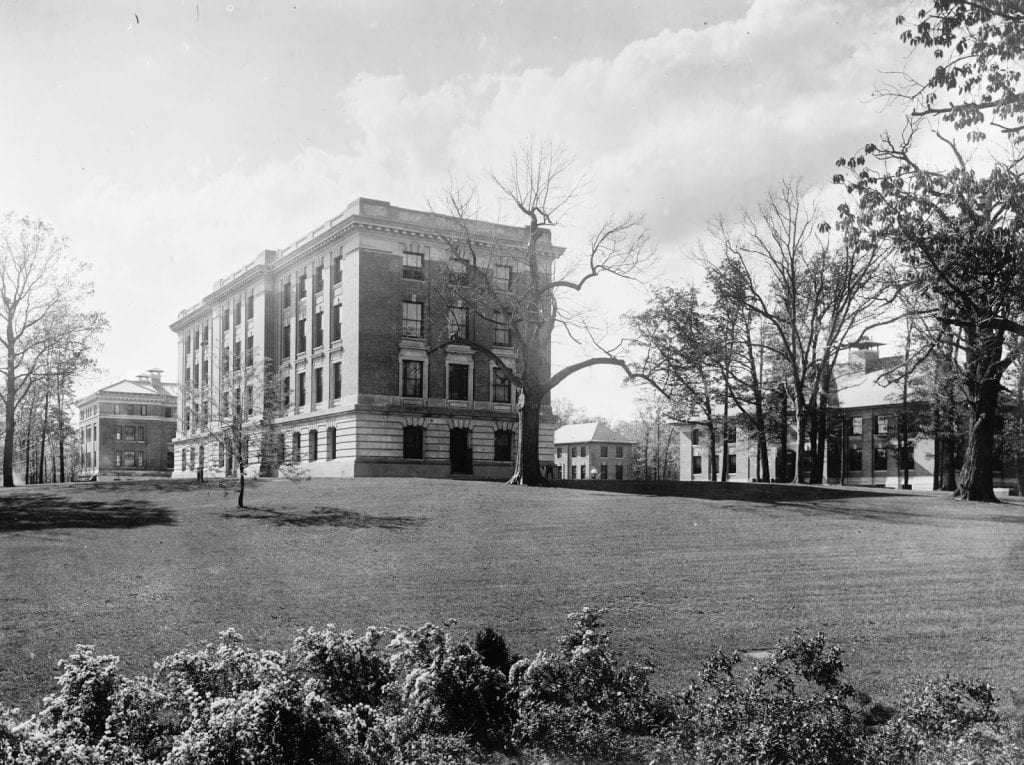
In the late 1950’s it was decided that NBS would move from its initial site on the outskirts of Washington DC to Gaithersburg, MD.  According to De Ferrari [DF13] “The Bureau’s director testified to Congress in 1956 that the Van Ness location was no longer tenable, in part because it was “extremely vulnerable in the event of an atomic attack.””. Gradually, the old buildings (Figs 18, 19) were left behind and the NBS reassembled in its new location where construction was mostly complete by 1970.  None of the 90 original buildings was preserved.

At some point in the 1970’s, the decision was made not to move the 4.5 ft wind tunnel, and it was offered to John Laufer, the inaugural chair of the USC Department of Aerospace Engineering. 

Laufer had worked with von Karman at Caltech, where he earned his PhD, and in 1949 he went to NBS to work in the group of Dryden and Schubauer.  In 1952 he moved to JPL, and took up his new position at USC in 1964.  It seems fitting that the NBS wind tunnel found its new home in Southern California and with John Laufer.  Here it was officially named the Dryden Wind Tunnel.

1976 – mid-1990’s: classic experiments at USC

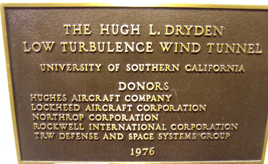
The Dryden Wind Tunnel (DWT) was officially inaugurated in 1976 (Fig. 21).

The DWT was to host numerous important experiments on turbulence and turbulent boundary layers, and experiments there became well-known for the use of multiple hot-wire rakes.  The first report of such experiments was by Blackwelder and Kaplan in a 1976 paper ‘On the wall structure of the turbulent boundary layer’ [Bl76].  Note that this work was on the spatial structure of a fully-developed boundary layer and was hosted in a different 2’ x 3’ tunnel where the boundary layer was deliberately tripped, so the details of transition to instability and turbulence were by-passed.  The personnel and techniques were as used in DWT as it came online for many years.

Figs 22 & 23 show the hot-wire rakes, which were custom-made.  Their fabrication by the principals involved and by associated graduate students and postdocs became a characteristic feature of the USC experimental facilities.

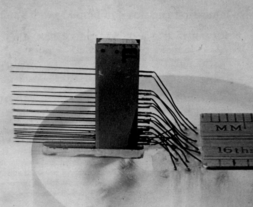
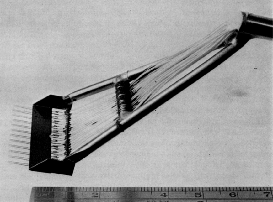
Fig 24 shows an example of the output from the 10 hot-wire traces in the wall-normal direction, y.  One or two technical details may be worth noting.  First, it is not completely easy to manufacture a multi-wire rake – and have all channels working, and have them working for a whole experiment.  The platinum wires are strong, but thin, with an estimated diameter of 2.5 um.  Obtaining a figure such as Fig. 24 is thus a feat in itself.  Second, the data acquisition and analysis were quite sophisticated at the time, as all 12 analog signals were recorded on a 14 channel analog magnetic tape recorder.  A second identical tape drive was used to replay the signals which were then converted through a 16-channel simultaneous sample-and-hold analog to digital converter.  The digital data were then analysed on a minicomputer with custom programs.  Third, note that the traces look quite different from those obtained in a transitioning boundary layer; there are no calm periods between bursts, and the boundary layer is fully turbulent.  Fourth, it is obvious that there is coherence between neighboring hot-wire signals, and it is reasonable to wonder whether that structure is related to the original spots observed in transition, or whether they are marks of some other pattern.  It seems possible that there is pattern within the turbulence – in other words, a turbulent boundary layer is not just a mess of statistical turbulence.

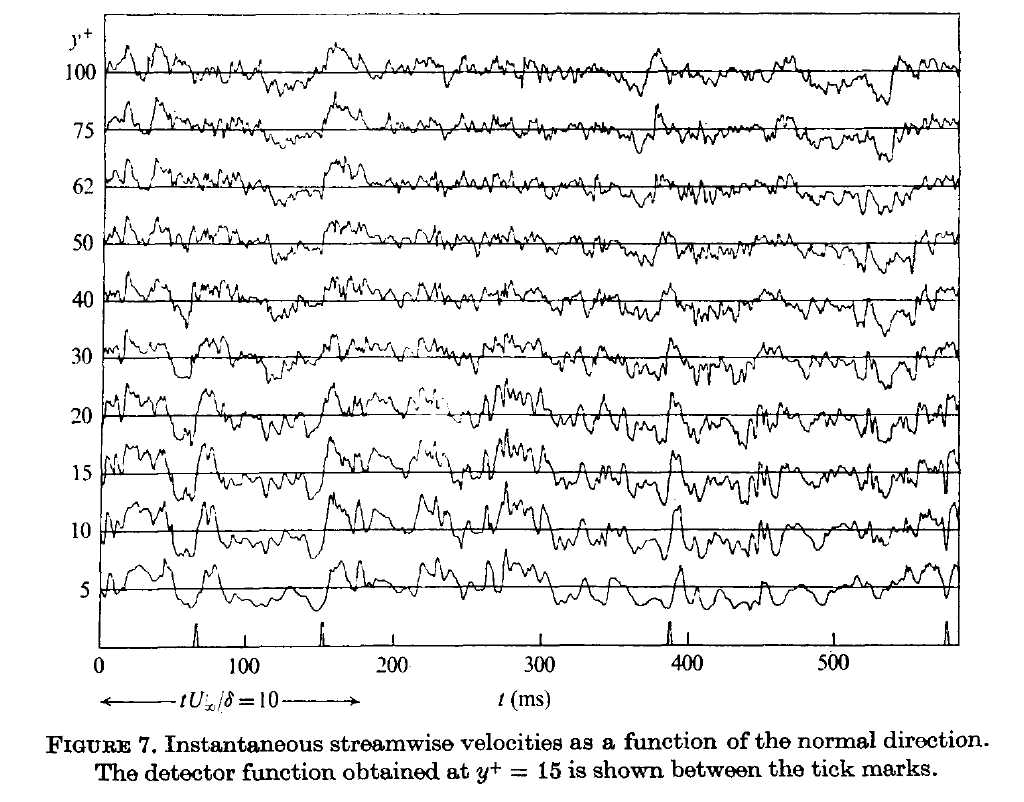
The fifth point is that [Bl76] used conditional sampling to process the data.  There are 4 heavy tick marks along the time axis of Fig 24 showing the location of a conditional sampling signal that was taken from the signal at y+ = 15.  One can see that these locations mark a high amplitude and clean zero crossing.  This was a most important aspect of the work as now the data could be interrogated based on certain criteria that were thought to indicate important dynamics.  We may revisit the idea of whether there is pattern and coherence in the turbulence.  Fig. 25 shows there is.

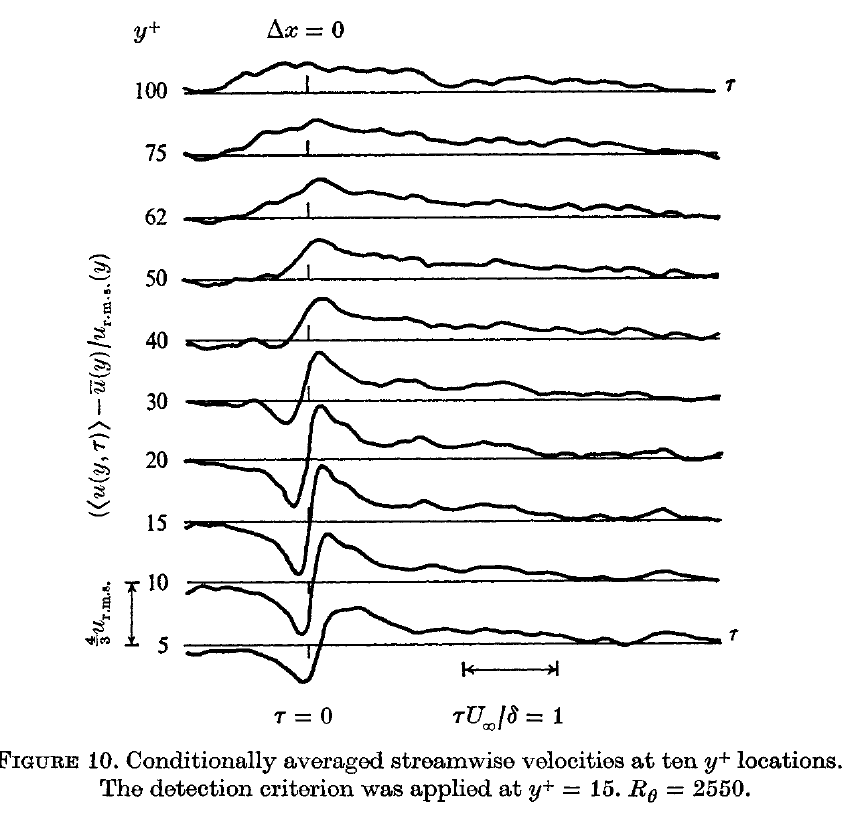
Fig. 25 shows the conditionally-averaged structure of wall turbulence.  It is not completely random.  The amplitude of the fluctuations near the wall is large but correlated compared with fluctuations in the outer flow.  It is possible that the turbulent fluctuations in the near-wall region drive the larger scale motions in the outer layer, allowing turbulence to regenerate.

Some further context comes from understanding the principal figures involved and the general research questions of the time.  Laufer had assembled a number of top names in emerging turbulence studies.  He himself had been responsible for pioneering already-classic research on the structure and statistics of turbulence in pipe and channel flow [La51, La54] where he applied new statistical theories of turbulence to experimental observations.  A common approach in the field was to decompose the flow into mean and fluctuating quantities and to consider various way in which to re-write the Navier-Stokes equations based on this decomposition combined with proposed models to simplify and model the products of fluctuating velocities.  These equations came to be known as the Reynolds-averaged Navier-Stokes equations (RANS).  Efficient computer codes based on these equations and models still form the foundation of industrial scale fluid mechanics computations, where the cost of simulating all spatial and temporal scales remains prohibitive.  The most direct application would be in central parts of turbulent pipe flow or of channel flow, but there were problems when near wall boundaries, when it was clear that at some point, the simplifying notion of isotropy could not be maintained.  Moreover, evidence was accumulating that coherent structures could exist within turbulence, which would defeat closure schemes predicated on simple relations of the Reynolds stress components (products of the fluctuating velocity components).

Laufer in 1975 wrote a review in the Annual Review of Fluid Mechanics [La75], noting the presence of structure in free-shear layers, wakes and jets, and in boundary layers.  One of the notable papers describing coherent features in boundary layers was by Blackwelder (Fig. 26) and Kovaszny (at Johns Hopkins).  Kaplan (Fig. 27) arrived at USC in 1964, following publication of his thesis at MIT.  The thesis was entitled ‘The stability of laminar incompressible boundary layers in the presence of compliant boundaries.’  Buried in this title is the impressive fact that Kaplan was the first to provide general numerical solutions to the Orr-Sommerfeld equation.  Up until that point solutions were only arrived at through quite technical asymptotic analysis which was required because certain modes of the solution grew much faster than others.  Kaplan designed a ‘purification’ scheme to separate out the fast- and slow-growing modes, and thus could solve the OS equations in a number of different configurations, which he did.  This included the original motivation, to investigate OS solutions for signs of drag reduction due to compliant (i.e. non-rigid) boundaries (following the suggestion of his thesis advisor Marten Landahl).

Blackwelder and Kaplan (encouraged and informed by Laufer and also by FK Browand, who had first observed periodic coherent structures in mixing layers [Br66, Wi74]) were thus perfectly poised to make significant contributions to the literature and to clarify the possible role of coherent structures in turbulent boundary layers.  The idea that turbulent was not necessarily a uniformly complex statistical jumble was exciting because it implied that further mechanical understanding outside statistics could emerge, with profound implications in turn, for control efforts.

Kaplan also took a special interest in computing and electronics, and soon USC DWT had one or the more powerful minicomputers on campus, a DEC PDP 11/55, with advanced facilities for conversion of analog signals and for their subsequent analysis.  Indeed, the Aerospace Engineering department had the first networked computer on campus, and a dedicated terminal room in a different building.  Memorably, one day when the computer was down, a hand-written note appeared on the door of this room: ‘Computer down.  Do theory.’

A further example of multiple hot-wire investigations in the boundary layer is given in Fig 28 from Wygnanski et al [Wi79].

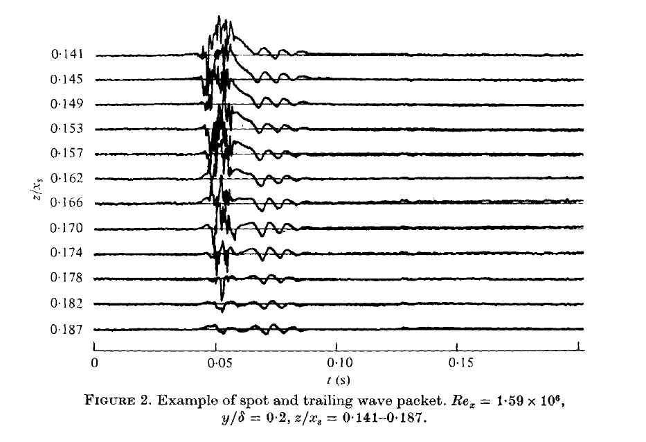
The study returned to the spatial structure of developing turbulence, and Fig 28 shows a multiple hot-wire reconstruction of a turbulent spot, with a wave packet in its lee.  Now the signals have been digitized they can be interrogated after the fact and ensemble averages can be constructed based on the wave packet timing.  Fig. 29 shows such an average.

The small-scale turbulence characteristics seen in Fig. 28 are washed out in the averaging, but the TS waves are clearly present and were determined to reside through the entire spot.  The turbulent spot and associated oblique wave packet were responsible for strong shear in both spanwise and normal directions, setting the seed for inflectional profile instabilities that cause the turbulence to grow.

1970 – 1990 New airfoil design and testing

Recall that one of the original motivations for the proper design of wind tunnels had been the difficulty in reconciling measurements on lift and drag for different shaped airfoils and at different facilities.  As the inviscid theories were brought into agreement with observations of nonzero lift and drag, it was becoming clear that measured airfoil characteristics did not always scale up well from the low Reynolds numbers of wind tunnel tests to the higher Reynolds numbers of actual flying machines.  One way of facing this challenge was to just make the wind tunnels bigger, culminating in the famous 80’ x 120’ tunnel at NASA Ames.  The problem with this approach was that it was much harder to control the flow quality, and a growing body of evidence continued to show that the appearance of turbulence led to very large variations in performance and that this transition depended quite strongly on the facility and its background turbulence levels.

The generation of families of airfoil shapes was well advanced beginning with the original Joukowsky airfoils obtained by conformal mapping techniques, and carrying systematic variations of camber and thickness.  The practical testing of these airfoils and wings was an essential element in qualifying shapes for practical uses and tables of lift, drag and moment coefficients sprang forth, e.g. Abbott & Doenhoff’s book entitled ‘Theory of Wing Sections’ [Ab59], which includes the following acknowledgement: “The authors also wish to acknowledge the contributions to the attainment of low-turbulence air-streams made by Dr. Hugh Dryden and his former coworkers at the National Bureau of Standards, …”.

Three sets of problems emerged.  The first was how to synthesize and test profiles that were derived from potential flow.  Second, how do results at (invariably) smaller scale translate up to full-scale?  Third, what are the boundary-layer and viscous effects and how may they be predicted and controlled?

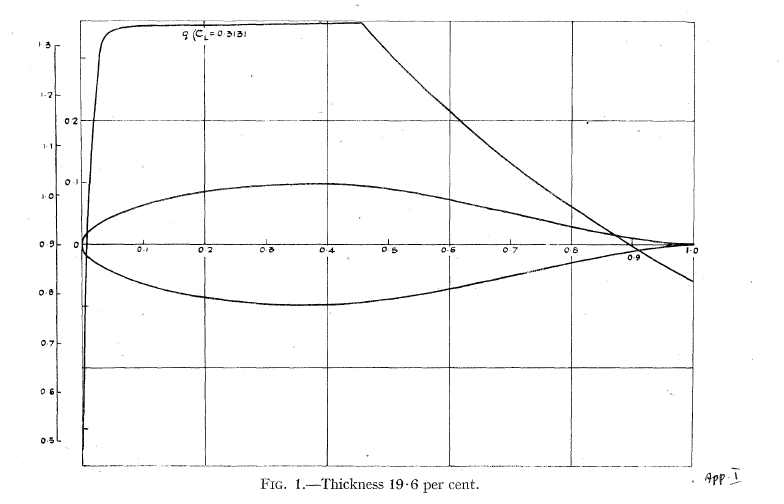
An alternative to building and testing families of profiles would be to run the design process backwards, beginning from a desired aerodynamic profile, back to a shape that would make it.  Lighthill [Li45] was the first to do this and showed a method that would start with a velocity distribution and then make an inverse design to a shape.  The technique took place in complex potential space and a Fourier series was used to map the velocity to shape coordinates (all the while retaining the Kutta condition at the trailing edge).  The basic derivation was completed in 2 concise pages and the remainder of the work was turned towards examining specific numerical examples of designs with different criteria.  The first example is shown in Fig. 30.

The Lighthill method was elegant and comparatively straight-forward, but did not include a systematic way of accounting at the design stage for viscous and possible separation effects.  Using matched asymptotics, Stratford in 1959 [St59] formulated a method for rapid estimation of separation of a turbulent boundary layer and an extension of this work showed how a pressure profile could be specified so that the boundary layer will be close to separation, but not beyond.  (He tested certain aspects of the theoretical development against the classical measurements of Schubauer and Klebanoff at NBS.) 

Liebeck and Ormsbee [Li70] were the first to combine Stratford’s solution for a pressure recovery region (in airfoil flows, the upper surface experiences a lower pressure but this must be matched with the higher pressure from the lower surface at the trailing edge.  The streamwise domain where the pressure must therefore increase is termed the pressure recovery region.) with no separation together with finding the shape that corresponds to the specified pressure distribution. 

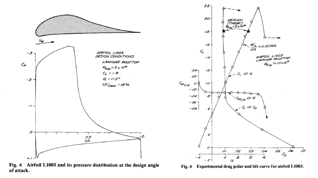
Initial formulations prescribed either an initial laminar boundary layer that abruptly transforms to a turbulent one, or for turbulent boundary layers from leading to trailing edge.  A number of airfoil sections with very high lift were produced (Fig. 31).

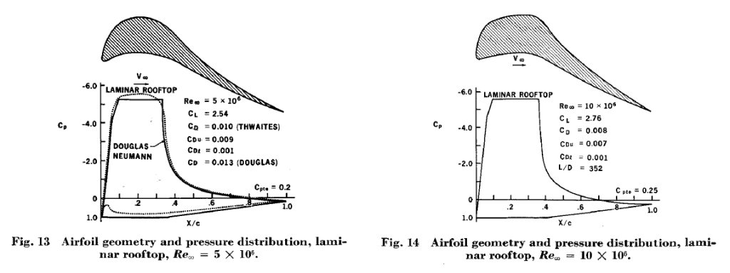
There is no guarantee that airfoil sections emerging from this calculation will be practical or buildable but the technique was powerful in that it led to shapes that would not likely have been encountered in parameter searches through airfoil families.  Nevertheless, the profile properties need to be tested and verified.  At the time Liebeck worked at the Douglas Aircraft Company, soon to become McDonnell Douglas, in Long Beach, and the first tests (Fig. 32) of the high-lift devices took place at the Douglas wind tunnel [Li78].  Designs included those specifically for high lift, and/or low drag, for compressible flows, for multi-element airfoils (flaps, slats) with target platforms ranging from high-altitude, long-endurance aircraft, sailplanes, propellers, fans, windmills, and for race cars.  In the latter case, the Liebeck-designed airfoil was on the car that won the Indianapolis 500 in 1975.

By 1978 Liebeck (Fig. 33) was an adjunct professor at USC and began a collaboration with Blackwelder that lasted a number of years.  It was only natural that attention would turn toward viscous boundary layer effects and how they might influence inverse airfoil design.  One example from this period illustrates several threads encountered already. 

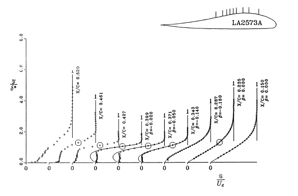
PhD student Pat LeBlanc together with Blackwelder and Liebeck used the DWT to measure properties of the LA2573A airfoil at Re = 235000.  Lift and drag were measured and hot wire surveys measured the boundary layer profiles along the suction surface of the airfoil.  At these comparatively low R, a laminar separation bubble (LSB) is almost an unavoidable feature.  In an LSB, a laminar boundary layer separates due to an increasing pressure in the streamwise direction, and the bubble plus TS waves then can be unstable, cause transition to turbulence, and then may reattach.  The effect of the LSB may be malign, negligible, or benign, depending on details of the geometry and R.

LeBlanc et al. carefully measured the velocity profiles above the airfoil (Fig. 34) and used the shape factors of the profiles to estimate growth rates in the Orr-Sommerfeld equations from equivalent Falkner-Skan boundary layer models (these are the classical Blasius solutions worked out under Prandtl but with the presence of a streamwise pressure gradient).  There was good agreement between the linear stability predictions of most amplified wave numbers and frequencies and their growth rate in both the laminar region and at the transition point.  The finding that observations were consistent with inviscid inflectional profile instabilities was quite important for future modeling efforts, where aeronautical calculations require TS, separation and transition prediction models.  These become increasingly important at low R, and in aeronautics R < 10⁶ is considered low.  It perhaps does not need pointing out that the low ambient turbulence levels of DWT were essential in this work.

The DWT focus thus returns full circle to studies of airfoils and wings, now armed with 70 years-worth of developments in both theory and experimental technique.  A final technical report of their research by Liebeck and Blackwelder [Li87] investigated the effects of ambient turbulence on LSBs, and the nature of instabilities around the bubble and transition point.  Fig. 35 shows spectra from the upper surface boundary layers.

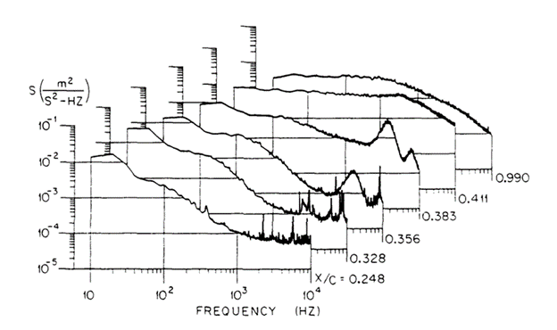
An experiment was then conducted where acoustic forcing from an internally-mounted loudspeaker was tuned to the natural frequencies of the LSB and transition region, as shown in Fig 34.  The result was a decrease in drag.  The boundary layer thickness at transition had decreased and the frequency peak had sharpened.  The quite far-reaching consequences of these observations were not pursued, but much later can be seen as the seeds for studies published about a quarter of a century later, again (or still!) from DWT experiments.

Clearly, the idea of manipulating the LSB as a means of flow control was promising and such an example is found in [Ke93] where vortex generators were embedded within the laminar boundary layer of a LA2573A airfoil at R between 200000 and 600000 (Fig. 36).

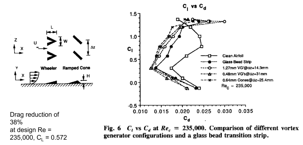
Systematic hot-wire surveys in {x,z} above the suction surface showed the contours of characteristic boundary layer profile heights, directly demonstrating the reduction in LSB height and concomitant reduction in turbulence intensity.

Vortex generators are by now commonly found on the upper surface of commercial aircraft, where the conditions are at much higher R.  This was the first demonstration of their efficacy (with > 30% possible drag reduction) at moderate R, and again with hindsight, these studies opened the door for later investigations of flow control at lower R.

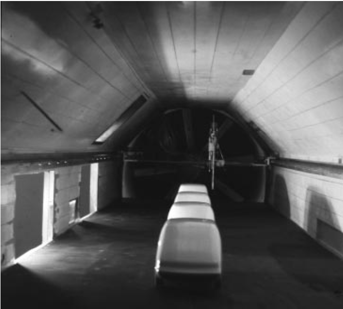
Mid-90’s – mid-2000’s: ground vehicle aerodynamics

In the mid-90’s, work in DWT transitioned (so to speak) to experiments on vehicle aerodynamics under the guidance of Fred Browand (Fig. 37), who we had previously mentioned in association with coherent structure formation in mixing layers.

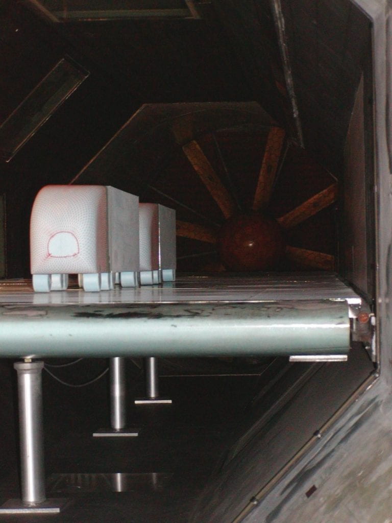
Fig. 38 shows the characteristic octagonal section of the DWT, now partially occupied by vehicle models and Fig 39 looks downstream with the tunnel fan blades visible.  There are certain obvious problems in conducting vehicle aerodynamics studies in a wind tunnel.  One relates to the problem of Reynolds number scaling.  It was found that with appropriate boundary layer trips, that the influence of varying R by a factor of 6 up to 5 x 10⁵ was small, within measurement uncertainty.  With attention to model geometry, results could be extrapolated out to the factor of 6-8 required for full-scale.  The second problem is that a vehicle moving over a fixed boundary does not see a boundary layer that necessarily accompanies an oncoming flow arriving at a fixed model.  The approach was to remove the boundary layer by suction from a slot close to the front face of the lead model (Fig. 39).  These details are examined in [Za95].

What followed then was a decade of publications detailing the aerodynamics of single, or more often groups, of vehicles.  The motivations were not difficult to understand.  As urban areas become increasingly dependent on ground vehicle transportation it becomes increasingly urgent to find ways to improve the cost of transport, reduce emissions and if possible to reduce crowding.

Building new freeways is lengthy, expensive and fraught with political and social hurdles.  Moreover, an extra lane on a freeway often just fills up, delivering yet more traffic to some other, already-saturated location.  Alternatively, one might imagine cars, vans and trucks under computer control so they could form a closely-spaced platoon in a special lane.  Vehicles could join upon request and with possession of the appropriate controller and software, and when in place would operate autonomously, without driver input.  Such coordinated control could lead to a much denser packing with considerably shorter distances between successive vehicles.  Now closer spacings are possible, what should they be from an energy-saving perspective?  Is there an optimum?

There is an optimum, Browand and colleagues determined, and it is set by the size of separation vortices.   2-4 vehicle platoons were measured to have about 55% of the drag in isolation.  Longer platoons would save more [Za95]. Incidentally, the force balance measurements required the development of a very sensitive force balance, yet with damping of modes that would be excited by having the relatively high mass models attached.  The force balance (Fig. 40) became the mainstay of many sensitive aerodynamic measurements for the next 30 years.

The vehicle tests were extended to single and platooning truck-trailer combinations (Fig. 39), and energy-saving configurations for cab-trailer spacing, and for aft- or end-conditions were investigated.  Deflected plates, called base flaps, mounted to the trailing edge of a trailer could yield significant reduction in energy consumption (drag), and these can be seen on trucks operating in the US today.

The studies were conducted in concert with the California PATH program, UC Berkeley, Lawrence Livermore National Lab and the US Departments of Transportation and Energy [Ha04].  They also included field tests conducted in 2003 [Br03] on an unused airfield runway at the northern end of the San Joachin Valley, where drag reductions of 10-12% were realized with spacing between real trucks of about 10 m (about 0.6 trailer lengths).

Back to boundary layers

In [Ha04], the first results of digital particle image velocimetry (DPIV) measurements on the truck vehicles were described, marking a second major upgrade in DWT instrumentation.  The DPIV methods had been used previously in a return to fundamental fluids studies by Hammache, Browand and Blackwelder [Ha02] who investigated the performance of an axisymmetric body of revolution (think missile or torpedo) when the lee end was crafted as a Stratford recovery region (much as had been tested earlier in Liebeck airfoils [Li78]).

The Stratford recovery solution [St59] was designed by matching viscous boundary layer models with an outer inviscid flow, and was proposed as a solution for gradual pressure increase on an airfoil, while just marginally avoiding separation, and it was interesting to find out whether this solution also pertained to a non-lifting body, where the basic problem is: how does a volumetric body terminate with minimum drag?  [Ha02] found that the Stratford design worked much better than either more gradual or more abrupt slopes of the aft-body.  This information would be quite interesting to various Air Force and Navy interests, one may imagine.  As Fig. 41 shows, the ability to measure velocity components, at once, in an entire field of view, as opposed to data assembled through repeated surveys of single point sensors, was quite a step.

Mid-2000 – today: wings at low Reynolds number

John McArthur was a co-author in [Br04] on drag reduction in truck platoons, and had been encouraged by Blackwelder to pursue his interests in small-scale flying devices, or Micro Air Vehicles (MAVs).  At the same time, the DWT now had in operation an advanced DPIV system, using custom software that had been developed at USC [Fi97].  It was possible to measure velocity fields and their spatial gradients to good accuracy.  The custom-built force balance could also be tuned to operate over a small range of small forces, and the pieces were in place to make fresh studies in low Reynolds number aerodynamics.

Though most classical aerodynamics studies were concerned with flows at large scales and high speeds, with characteristic values of R well above 10⁶, and the properties of wings at much smaller scale were not well-established.  Though R is smaller, in the range R = 10⁴ – 10⁵, the viscous-inviscid interactions are extremely complex and in many cases, enormously sensitive to small disturbances.  Consequently, the technical literature was in a state of some disarray with disagreements on drag coefficients, for example, by factors of 2 or more.  Once again, the low turbulence characteristics of the DWT would be essential in making correct measures of airfoil and wing performance.  It was also a point of interest that the new domain of MAV aerodynamics overlapped in R-space with the natural flight of many birds and bats, and the custom DPIV techniques of [Fi97] had been brought successfully to a new wind tunnel in Lund, Sweden to investigate the flight of birds [Sp03].

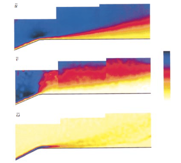
McArthur painstakingly measured well-resolved, overlapping DPIV fields to put together detailed maps of the complex, separated flow fields over wings/wing sections (Fig. 42).

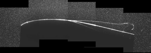
The time-averaged properties of the boundary layer could therefore be reconstructed.  DPIV methods enable instantaneous field measurements, and one such view is shown in Fig. 43.

There were numerous eye-opening data sets.  At these low R, aerodynamic performance is largely dictated by the resistance, or lack of it, to separation in the boundary layer, as noted years before by Lissaman [Li83], who had also joined the AE department at USC.  It was found that curved flat plates work better (have higher L/D) over all angles of attack than standard airfoil sections at R < 10⁵.

Further light was also shed on the abrupt changes in C_l(C_d) polars that characterize many airfoil sections at low R.  By approaching from a low R and gradually increasing it, a new family of polars was measured (Fig. 44).

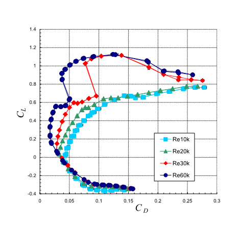
The curves for R = 30k and 60k are especially interesting as there are points on the lower envelope where the data suddenly jump to the upper envelope.  These jumps are accompanied by a reduction in C_D and a substantial increase in C_L.  The large change in forces coming from a small change in geometry (angle of attack, a) immediately suggest that flow control may be possible, and efficient.

Indeed, this proved to be the case, and a series of tests were conducted by PhD student Shanling Yang, using acoustic forcing, either global or local, to switch the flow from state SI to state SII.  In doing this we were unwittingly following the lead set by Liebeck and Blackwelder [Li87] 26 years previously, and also leveraging the early results of Schubauer and Skramstad [Sc37].

The two main differences can be seen in Fig. 45, where a rectangular array of miniature speakers forces the flow locally, and the PIV methods allow the sectional flow field to be reconstructed.

In running these experiments, we accidentally found that simply having holes present was itself enough to switch the flow from SI to SII (Fig. 46).  It took more than 2 weeks of worry before understanding that the open holes and backing chambers for the wiring beneath were providing a cavity where Helmholtz resonance could, or rather would, occur.  In some sense, the wing was singing to itself, controlling the local aerodynamic forces.

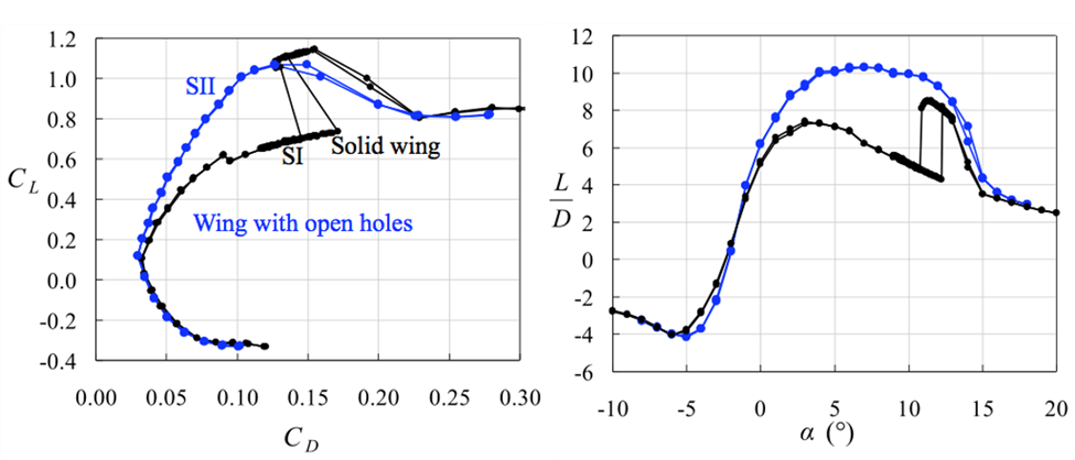
The largest changes in L/D (right panel of Fig. 46) occur close to (L/D)_max, so it would be a reasonable operation point for the wing/foil.  Current research is looking for ways to make an efficient feedback control system based on acoustic actuation.

Designing an airplane from scratch (J. Huyssen)

The first commercial aircraft having the properties we recognize today was the Douglas DC3, introduced in 1936.  It had a metal monocoque fuselage shell, a single pair of wings with metal skin and engine supports, and a tail plane mounted – well – at the tail.  The tail plane (or empennage) gives the plane passive stability in pitch.  The tube and wing (TW) design has remained unchanged for a little less than 90 years.  Does this mean it is optimal?  Could we do better?  By what standard?  Is there an optimum configuration?  These are quite difficult questions to answer, and PhD student Joachim Huyssen has been addressing them in a quantitative way.  The path from armchair engineering design, to testing to conclusions is shown in Fig. 47.

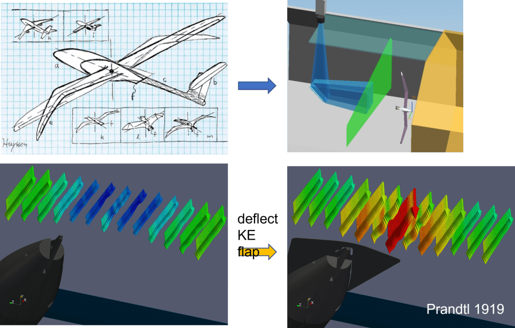
In inviscid theory the optimal wing is loaded (has a local circulation distribution) elliptically, or close to it.  This produces a constant downwash, and one can show that any departure from this flat function conveys less vertical momentum flux per unit energy, and so must be inferior.  Inserting a fuselage cannot be good from this point of view. 

Instead, Huyssen set about wondering how the flow around a different-shaped fuselage might be tailored aerodynamically.  In theory, a flat-plate flap mounted at the aft end of the fuselage could modify the separation location, and hence the circulation, on the body to match what it would have been had the body not been there.  This device was termed a Kutta-Edge flap because it moves the point where the Kutta condition is applied for finite lift in an inviscid calculation. In 2010, Huyssen made a series of tests using PIV methods in the DWT.  Some are shown in the lower row of Fig. 47, where the bottom line is that the KE arrangement does work.  The DWT results are given in [Hu12]. The topic is quite complex, and lengthy.  [Hu16] showed how a quantitative measure called an Inflation Factor (IF) can be constructed, which measures the magnitude of departure of a given configuration from a hypothesized ideal wing.  The TW is further from an optimum than the KE configuration.  Based on this information alone, we may conclude at the very least that further exploration of this topic is justified, if not morally mandated in times of increasing stress on the environment.  To be continued.

Surprises in wing performance at small scale – we know less than we think

As last updates on work from the DWT, we return all the way back to airfoil performance.  Given that so much of the technical literature on low Reynolds number aerodynamics is in an uncertain state, it was decided to carefully measure the lift and drag on an aerodynamic standard – the NACA 0012 airfoil.  This symmetric airfoil is in all the textbooks and its properties are well understood at high R.  It turned out not to be the case at lower R (Fig. 48).

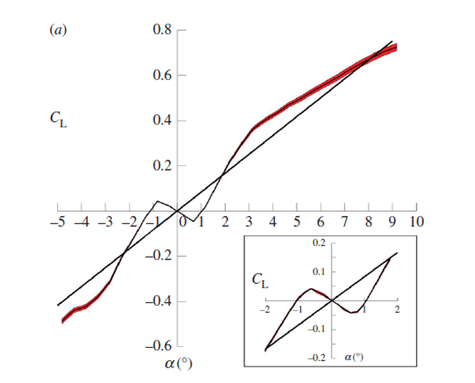
Let us begin at a = 0, where C_l = 0, as it should be for a symmetric airfoil.  As a increases the lift now goes negative, so the slope of C_l vs. a (upon which control algorithms are based) is the reverse of what is expected.  The slope then switches sign and there is a high, positive dC_l/da. Over the range of a = 2 -7 degrees, the airfoil does better than theory.  At higher a the stall is very gradual.  The cause is the shifting of separation points on the upper and lower surfaces, as the flow always separates before the trailing edge at these low R.  Combined PIV studies demonstrate these movements [Ta17].

Why was this such a surprise?  Why has this phenomenon not been seen before?  It seems that no previous measurements on this shape at this or similar R have had at their disposal the powerful combination of a genuinely low-turbulence wind tunnel and a sophisticated and sensitive strain-gauge load cell.

The curious shape of C_l(a) in Fig. 48 derives from careful measurement of a rather plain vanilla airfoil, and there is no reason to believe that a range of airfoils and wings of similar or greater thickness will not behave the same way – if only sufficiently careful measurements are taken. 

Given that such exquisite care needs to be taken to establish nicely-ordered flow conditions to observe and understand the geometry of shifting separation points, it could be that the nonlinear lift curve is not general in practical devices which do not necessarily fly in perfectly still air.  It is interesting to consider that wings of this size overlap in R with birds and bats, and then to wonder how they work.  Bird wings, for example, are flapped through high amplitudes, are flexible, and porous. 

Suppose we add one ingredient to the NACA 0012 baseline case, and add porosity, all other things being kept the same.  The result is in Fig. 49, compiled by PhD student Yohanna Hanna.

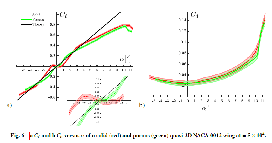
An array of 1 mm diameter holes was embedded in a second printed (and smoothly finished) NACA 0012 model.  The nonlinear behavior disappears.  Birds need not worry, and perhaps neither should we, as there seems to be no significant drag penalty for having the holes present.  There is a possibility that hole-design can be combined with the acoustic forcing (active or passive) ideas to make new wings for this scale of flight.

The ability to measure small forces, and variations in these small forces, together with accurate PIV methods for estimating velocity fields and their gradients remain the core of DWT operations today.  The tunnel was originally designed for transitional boundary layers.  Now as we wish to understand the properties of small wings, each wing has a potentially transitioning boundary layer and laminar separation bubble, and the facility still positions us uniquely to advance our understanding of these sensitive and complex flow.

Parting thoughts

There are a number of themes that run through this historical account of the journey of the NBS wind tunnel to its current DWT form.  I would like to outline two.

It may strike the reader that the progress through our understanding of turbulence, from combined experimental, analytical and theoretical investigations, has been very slow.  We have traced the wind tunnel evolution from transition in a laminar boundary layer through to seemingly an endless supply of questions as to where and how a general theory of turbulence might be constructed.  Issues of spatial and temporal intermittency and the universality of similarity solutions in shear-dominated flows recur.  Over the same time period, say from 1910 – 1980, we have developed quantum mechanics, special and general relativity, big-bang and multiverse theories of cosmology, we have gone to the moon (and back),and invented the transistor, digital computers and the internet.  Why are we so slow?  In retrospect this seems like a fair question, but it is striking in reading the source literature that fluid turbulence admits only grudgingly to novel ideas and hypotheses, and each one of these must be tested with care and rigor.  The literature that we have just skimmed over is a magnificent record of original, thoughtful and inventive work by a gradually growing army of scientists and engineers.  Each new thought demands testing and checking, sometimes in multiple ways.  We have been slow because the problem is hard, but the intellectual achievements and people involved have been of the very highest caliber.

This leads to the second, more personal, thread, where I have greatly enjoyed following the traces of people and ideas from the early 20^th century (or before), on to experiencing the facilities, techniques and people first-hand at USC.  It has been my privilege to have known many of the more recent main actors in the drama of turbulence and fluid mechanics as colleagues and mentors, and it has been exciting and enthralling to be immersed in this historical reconstruction.  I now have a better idea of where I am, and I hope some who read this account will too.

GR Spedding  5/24/2023

References

[clicking on the [Abxx] tag will often bring up directly the PDF of the file.]

[Ab59] Abbott IH & von Doenhoff AE 1957 Theory of Wing Sections. Dover, New York.

[Bl76] Blackwelder RF & Kaplan RE 1976 On the wall structure of the turbulent boundary layer. J. Fluid Mech, 76, 89-112.

[Br59] Briggs LJ 1959 Effect of spin and speed on the lateral deflection (curve) of a baseball; and the Magnus effect for smooth spheres. Am. J. Phys. 27, 589-596.

[Br66] Browand FK 1966 An experimental investigation of the instability of an incompressible, separated shear layer. J. Fluid Mech. 36, 281-307.

[Br04] Browand FK, McArthur J & Radovich CR 2004 Fuel saving achieved in the field test of two tandem trucks. Calfornia PATH Research Report UCB-ITS-PRR 2004-20.

[DF13] De Ferrari 2013 Streets of Washington. http://www.streetsofwashington.com/2013/07/the-lost-hilltop-home-of-national.html

[Dr20] Dryden HL 1920 Air forces on circular cylinders, axes normal to the wind, with special reference to dynamical similarity. NBS TR 394.

[Dr26] Dryden HL & Heald RH 1926 Investigation of turbulence in wind tunnels by a study of the flow about cylinders. NBS TR 231

[Dr29] Dryden HL & Kuethe AM 1929 The measurement of fluctuations of air speed by the hot-wire anemometer. NACA TR 320.

[Dr36] Dryden HL, Schubauer GB, Mock WC & Skramstad 1936 Measurements of intensity and scale of wind tunnel turbulence and their relation to the critical Reynolds number of spheres. NBS TR 581.

[Dr48] Dryden HL & Abbott IH 1948 The design of low-turbulence wind tunnels. NACA TR 940.

[Fi97] Fincham AM & Spedding GR 1997 Low-cost, high resolution DPIV for measurement of turbulent fluid flow. Exp. Fluids 23, 449-462.

[Fr67] Frenkiel FN & Klebanoff PS 1967 Correlation measurement in a turbulent flow using high-speed computing methods. Phys. Fluids 10, 1737-1747.

[Fr71] Frenkiel FN & Klebanoff PS 1971 Statistical properties of velocity derivatives in a turbulent field. J. Fluid Mech. 48, 183-208.

[Fr75] Frenkiel FN & Klebanoff PS 1975 On the lognormality of the small-scale structure of turbulence. Boundary-Layer Meteorology 8, 173-200.

[Ha02] Hammache M, Browand FK & Blackwelder RF 2002 Whole-field velocity measurements around an axisymmetric body with a Stratford-Smith pressure recovery. J. Fluid Mech. 461, 1-24.

[Ha04] Hammache M & Browand FK 2004. On the aerodynamics of tractor-trailers. In The aerodynamics of heavy vehicles: trucks, buses, and trains (pp. 185-205). Springer, Berlin Heidelberg.

[Ha19] Hanna YGT & Spedding GR 2019 Aerodynamic performance improvements due to porosity in wings at moderate Re. 2019 AIAA Aviation and Aeronautics Forum and Exposition, 17-21 June 2019, Dallas, Texas. AIAA 2019-3584.

[He22] Heisenberg W 1922 Absolute dimensions of Karman vortex motion. NACA TR 126.

[He24] Heisenberg W 1924 Uber Stabilitat und Turbulenz von Flussigkeitsstromen.” Annalen der Physik, Band 74, No. 15 (reprinted as “On the stability and turbulence of fluid flows” NACA TM 1291, 1951)

[Hu12] Huyssen RJ, Spedding GR, Mathews EH & Liebenberg L 2012 Wing-body circulation control by means of a fuselage trailing edge. J. Aircraft 49 (5), 1279-1289.

[Hu16] Huyssen RJ, Mathews EH Liebenberg L & Spedding GR 2016 On the wing density and the Inflation Factor of aircraft. Aero. J. 120, 291-312

[Ka64] Kaplan RE 1964 The stability of laminar incompressible boundary layers in the presence of compliant boundaries. MIT Thesis.

[Kl55] Klebanoff PS 1955 Characteristics of turbulence in a boundary layer with zero pressure gradient. NACA TR 1247.

[Kl62] Klebanoff PS, Tidstrom KD & Sargent LM 1962 The three-dimensional nature of boundary-layer instability. J. Fluid Mech. 12 1-34.

[Kl72] Klebanoff PS & Tidstrom KD 1972 Mechanism by which a two-dimensional roughness element induces boundary-layer transition. Phys. Fluids 15, 1173-1188.

[La07] Lanchester FW 1907 Aerodynamics, constituting the first volume of a complete work on aerial flight. London, Constable.

[La51] Laufer J 1951 Investigation of turbulent flow in a two-dimensional channel. NACA TR 1053.

[La54] Laufer J 1954 The structure of turbulence in fully developed pipe flow. NACA TR 1174.

[La75] Laufer J 1975 New trends in experimental turbulence research. Ann. Rev. Fluid Mech. 7, 307-326.

[Le86] LeBlanc P, Blackwelder RF & Liebeck RH 1986 A comparison between boundary layer measurements in a laminar separation bubble flow and linear stability theory calculations. In ‘Low Reynolds Number Aerodynamics’, Lecture Notes in Engineering vol 54, Springer, pp 189-205.

[Li70] Liebeck RH & Ormsbee AI 1970 Optimization of airfoils for maximum lift. J. Aircraft 7. 409-415.

[Li78] Liebeck RH 1978 Design of subsonic airfoils for high lift. J. Aircraft 15, 547-561.

[Li87] Liebeck RH & Blackwelder RF 1987 Low Reynolds Number – Separation Bubble. Final Technical Report AD-A199-378

[Li45] Lighthill MJ 1945 A new method of two-dimensional aerodynamic design. Reports and Memoranda of the Aeronautical Research Council, No. 2112

[Li83] Lissaman PBS 1983 Low Reynolds-number airfoils. Ann. Rev. Fluid Mech. 15. 223-239.

[Ma53] Magnus G 1853 On the deviation of projectiles, and: on a sinking phenomenon among rotating bodies. Annalen der Physik 164, 1-29.

[Mc08] McArthur J 2008 Aerodynamics of wings at low Reynolds numbers: boundary layer separation and reattachment. USC AME PhD Thesis.

[Pr04] Prandtl 1904. On fluid motions with very small friction. Verhldg, 3, 484-491.

[Ra77] Rayleigh 1877 On the irregular flight of a tennis ball. Messenger of Mathematics, VII, 14-16.

[Sc29] Schlichting H 1929 Zur Enstehung der Turbulenz bei der Plattenströmung”. Nachrichten der Gesellschaft der Wissenschaften – enshaften zu Göttingen, Mathematisch – Physikalische zu Göttingen, Mathematisch – Physikalische Klasse, 21-44

[Sc46] Schubauer GB & Klebanoff PS 1946 Theory and application of hot-wire instruments in the investigation of turbulent boundary layers. ACR 5K27.

[Sc47] Schubauer GB & Skramstad HK 1947 Laminar boundary-layer oscillations and stability of laminar flow. J. Aero. Sci. 14, No. 2., 69-78.

[Sc50] Schubauer GB, Spangenberg WG & Klebanoff PS 1950 Aerodynamic characteristics of damping screens. NACA TN 2001.

[Sc55] Schubauer GB & Klebanoff PS 1955 Contributions on the mechanics of boundary-layer transition. NACA TR 1289

[Sp03] Spedding GR, Rosén M & Hedenström A 2003 A family of vortex wakes generated by a thrush nightingale in free flight over its entire range of flight speeds. J. Exp. Biol. 206, 2313-2344

[Sp10] Spedding GR & McArthur J 2010 Span efficiencies of wings at low Reynolds number. J. Aircraft 47, 120-128.

[St59] Stratford BS 1959 The prediction of separation of the turbulent boundary layer. J. Fluid Mech. 5, 1-16.

[Ta17] Tank J, Smith L & Spedding GR 2017 On the possibility (or lack thereof) of agreement between experiment and computation of flows over wings at moderate Reynolds number. J. R. Soc. Interface Focus 2017 7 (1) 20160076.

[To29] Tollmien W 1929 Über die Entstehung der Turbulenz. 1. Mitteilung, Nachr. Ges. Wiss. Göttingen, Math. Phys. Klasse 21ff

[To31] Tollmien W 1931 Grenzschichttheorie, in: Handbuch der Experimentalphysik IV,1, Leipzig, S. 239–287.

[Wi74] Winant C & Browand FK 1974 Vortex pairing: the mechanism of turbulent mixing-layer growth at moderate Reynolds number. J. Fluid Mech. 63, 237-255.

[Wy79] Wygnanski I, Haritonidis JH & Kaplan RE 1979 On a Tollmien-Schlichting wave packet produced by a turbulent spot. J. Fluid Mech. 92, 505-528.

[Ya13] Yang SL & Spedding GR 2013 Passive separation control by acoustic resonance. Exp. Fluids 54, 1603

[Ya14] Yang SL & Spedding GR 2014 Local acoustic forcing of a wing at low Reynolds numbers. AIAA. J. 52, 2867-2876

[Za95] Zabat MA, Stabile NS, Frascaroli, S & Browand FK 1995 The aerodynamic performance of platoons: final report. California PATH Research Report, UCB-ITS-PRR-95-35.